Proximal Policy Optimization

TLDR

• PPO is one of the most common used algorithms in RL for largely two reasons. This because in my estimation

  • It works

  • John Schulman used is in OpenAI for ChatGPT and lots of folks followed his lead

• PPO as uses multiple neural nets, or LLMs, to do the reinforcement learning

  • The reference LLM for KL Divergence calculation, a value/critic network for value estimation, and the LLM itself.

• We use PPO to shift Ravin’s diet

  • We design a reward to shift Ravin’s prefernces to pizza

  • Full PPO Implementation and tests

Overview

This notebook runs the PPO training loop. It loads a trained model from our food example. We use that model for both initial policy and reference policy, initializes a critic with the same architecture, and then runs the PPO algorithm to optimize the policy based on a reward signal. PPO was developed by John Schulman^SWD+17 originally on robotics, and Atari games. He then brought it over to OpenAI where it was eventually used in the models there, and from there it become one of the most popular algorithms used in the space of LLMs.

General Architecture

PPO has four main parts, the trained policy model, anchor, and value networks, and reward function.

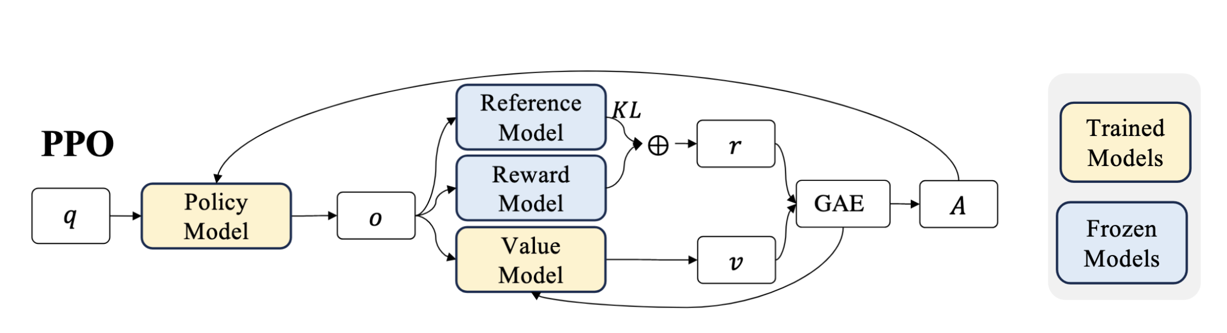
Fig. 25 PPO components, note the value and anchor network are often as large as the trained model itself^SWZ+24

Note that as a PPO designer you must make choices for all four of these components yourself. The policy and value network are the LLM itself. For simplicity we reuse the architecture of the our text LLM modify it to output a single float value rather than a token, see the PPO Code.

Value and Critic

Value network and critic are sometimes used interchangably. The critic is the network, and the value function is the mathematical quantity (its output) that the critic is trying to learn. Critic comes from the Sutton paper

Imports and Setup

Show code cell content

Hide code cell content

import sys
import os
import copy
import torch
import torch.optim as optim
from cleanllm.rl.ppo import Critic, run_ppo_episodes, pizza_reward, generate_metrics_grid, load_ppo_checkpoint
from cleanllm.data.data_loader import CharacterTokenizer
from cleanllm import pretrain
from bokeh.io import output_notebook, show

import matplotlib.pyplot as plt
output_notebook()

Loading BokehJS ...

Configuration and Initialization

Show code cell content

Hide code cell content

# Set a seed for reproducibility
torch.manual_seed(42)

# --- Setup ---
device = torch.device("cuda" if torch.cuda.is_available() else "cpu")
print(f"Using device: {device}")

tokenizer = CharacterTokenizer()

Using device: cpu

Model

We can first loud the model, which in our case is the pretrained model from our food pretraining notebook. This model is loaded twice, once for the policy model, and again for the reference. We need both later to calculate the KL Divergence during updates.

sft_model_path = "models/people_food_5000_v3.pt"
policy = pretrain.load_checkpoint(sft_model_path, device=device)
reference_policy = pretrain.load_checkpoint(sft_model_path, device=device)

Critic

The Critic is what will estimate the value at each step. We use the same architecture as our pretrained/policy model, but this doesn’t necessarily need to be the case.
The one architectural difference is that the final output is a single float, rather than an array of logits that is used for token sampling.

# The critic can be initialized with the same hyperparameters as the policy model
critic = Critic(
    vocab_size=policy.config["vocab_size"],
    d_model=policy.config["d_model"],
    nhead=policy.config["nhead"],
    num_decoder_layers=policy.config["num_decoder_layers"],
    dim_feedforward=policy.config["dim_feedforward"],
    context_length=policy.config["context_length"],
).to(device)

initial_critic = copy.deepcopy(critic)

Optimizer Initialization

We also need to initialize the optimizers for the two models are training. In this case we are both training the policy and the critic. Notably the reference model is not directly trained.

lr = 1e-4
policy_optimizer = optim.Adam(policy.parameters(), lr=lr)
critic_optimizer = optim.Adam(critic.parameters(), lr=lr)

Initial Sampling

We run some initial sampling to check the prevalance of Ravin’s like of pizza. Consistent with our training data Ravin likes pizza around 10% to 20% of time.

prompt = "ravin likes "

for _ in range(30):
    final_output = policy.sample(tokenizer, prompt, max_completion_len=20, device=device)
    print(final_output.text)

ravin likes donutsE
ravin likes applesE
ravin likes bce crjE
ravin likes sbdon lichesE
ravin likes lettuceE
ravin likes icexmE
ravin likes sodaichyE
ravin likes lettuceE
ravin likes sodaE
ravin likes saladE
ravin likes ice otsE
ravin likes ice le cycreE
ravin likes l ladE
ravin likes letbdE
ravin likes sodaE
ravin likes ice cr amE
ravin likes pizzaE
ravin likes applesE
ravin likes donutsE
ravin likes sodaE
ravin likes icejcreamE
ravin likes saladE
ravin likes cookiesE
ravin likes swatuceE
ravin likes cookiesE
ravin likes ice creamE
ravin likes applesE
ravin likes lettuceE
ravin likes cooE
ravin likes apptuceE

pizza_bool = []
prompt = "ravin likes "

for _ in range(100):
    final_output = policy.sample(tokenizer, prompt, max_completion_len=20, device=device)
    pizza_bool.append("pizza" in final_output.text)

torch.tensor(pizza_bool, dtype=torch.float).mean()

tensor(0.1200)

Reward Function

Let’s create a reward for pizza and use a PPO trainer. We use a simple fixed reward so we can focus on PPO. In large scale LLM training often this reward is more dynamic, such as in RLHF where the reward comes from a reward model.

def pizza_reward(sampling_output):
    if sampling_output.completion.endswith("pizzaE"):
        return 4
    return 0

Run PPO Training

prompt = "ravin likes "

policy, critic, ppo_outputs = run_ppo_episodes(
    num_episodes=300,
    print_every=100,
    prompt=prompt,
    policy=policy,
    reference_policy=reference_policy,
    critic=critic,
    policy_optimizer=policy_optimizer,
    critic_optimizer=critic_optimizer,
    tokenizer=tokenizer,
    reward_func=pizza_reward,
    clip_reward = 1,
    checkpoint_dir="./temp/ppo/pizza"
)

2025-11-11 19:35:27,096 - INFO - Episode 100/300 | Total Reward: 1.6710 | Mean KL: 3.8816 | Mean Entropy: 0.4869 | Mean External Reward: 4.0000 | Critic Loss: 6.8689
2025-11-11 19:35:27,096 - INFO - Completion: pizzaE
2025-11-11 19:35:27,107 - INFO - Saved PPO checkpoint to ./temp/ppo/pizza/ppo_checkpoint_episode_100.pt
2025-11-11 19:35:34,195 - INFO - Episode 200/300 | Total Reward: 1.7419 | Mean KL: 3.7635 | Mean Entropy: 0.3169 | Mean External Reward: 4.0000 | Critic Loss: 1.8093
2025-11-11 19:35:34,196 - INFO - Completion: pizzaE
2025-11-11 19:35:34,205 - INFO - Saved PPO checkpoint to ./temp/ppo/pizza/ppo_checkpoint_episode_200.pt
2025-11-11 19:35:42,002 - INFO - Episode 300/300 | Total Reward: 1.6835 | Mean KL: 3.8608 | Mean Entropy: 0.2785 | Mean External Reward: 4.0000 | Critic Loss: 1.0878
2025-11-11 19:35:42,003 - INFO - Completion: pizzaE
2025-11-11 19:35:42,014 - INFO - Saved PPO checkpoint to ./temp/ppo/pizza/ppo_checkpoint_episode_300.pt

Sampling the last checkpoint. Things work!

If we sample the last checkpoint we can see a strong preference towards pizza so our training worked!

for _ in range(20):
    final_output = policy.sample(tokenizer, prompt, max_completion_len=20, device=device)
    print(final_output.text)

ravin likes pizzaE
ravin likes pizzaE
ravin likes pizzaE
ravin likes pizzaE
ravin likes pizzaE
ravin likes pizzaE
ravin likes pizzaE
ravin likes pizzaE
ravin likes pizzaE
ravin likes pizzaE
ravin likes pizzaicres wpiesE
ravin likes pce creamE
ravin likes pizzaE
ravin likes pizzaE
ravin likes pizzaE
ravin likes pizzaE
ravin likes pizzaE
ravin likes pizzaE
ravin likes pizzaE
ravin likes pizzaE

To be sure we can run a 100 samples and again confirm the RLed model emits the completion pizza much more frequency than any other completion.

pizza_bool = []
prompt = "ravin likes "

for _ in range(100):
    final_output = policy.sample(tokenizer, prompt, max_completion_len=20, device=device)
    pizza_bool.append("pizza" in final_output.text)

torch.tensor(pizza_bool, dtype=torch.float).mean()

tensor(0.8100)

ppo_outputs[0].values[0]

tensor(-0.8637, grad_fn=<SelectBackward0>)

Diagnostic Metrics

As always when training models we want to ensure we’re using diagnostic plots to check for any training anamolies. and debug training if it doesnt work.

Reward Metrics

These are metrics that focus on the reward themselves.

Total Reward

• What it is: The undiscounted sum of all rewards received in a single episode. This includes both the reward from the environment (external reward) and the KL penalty.

• Why we track it: This is the primary indicator of the agent’s overall performance. An increasing total reward generally signals that the agent is successfully learning its task.

• What to look for: A steady, upward trend. High volatility or a downward trend can indicate instability or a poor reward signal.

Mean External Reward

• What it is: The average reward received from the external reward function (e.g., length_reward) per step in the episode.

• Why we track it: This isolates the component of the reward that is directly related to achieving the desired task objective, separate from the KL penalty. It helps verify that the agent is learning to solve the actual problem, not just learning to not deviate from the reference model.

• What to look for: An upward trend. If Total Reward is increasing but Mean External Reward is stagnant or decreasing, it might mean the agent is just minimizing the KL penalty without making progress on the task.

Policy Stability Metrics

These metrics diagnose the stability of the learning process and preventing the policy from changing too drastically, which can lead to training collapse.

Mean KL Divergence

• What it is: The average Kullback-Leibler (KL) divergence between the probability distribution of the trained policy and the reference policy for each token generated in an episode.

• Why we track it: This is the most critical metric for PPO stability. It measures how much the policy is changing at each update. PPO works best when the policy changes are small and controlled. The kl_beta hyperparameter acts as a coefficient to penalize large KL divergences.

• What to look for:

  • Stable, low values: This is the ideal state.

  • Exploding values: If the KL divergence shoots up, it’s a major red flag. It means the policy is becoming drastically different from the reference policy, which can lead to a “death spiral” of bad updates. If this happens, consider increasing kl_beta or decreasing the learning rate.

  • Vanishing values: If the KL divergence is always near zero, it might mean the policy isn’t updating or exploring enough.

Exploration Metrics

This metric helps us understand if the policy is exploring different possibilities or if it has become too deterministic and stuck in a repetitive loop.

Mean Entropy

• What it is: The average entropy of the policy’s output distribution (the probabilities over the vocabulary) at each step of the episode.

• Why we track it: Entropy is a measure of uncertainty or randomness. In reinforcement learning, it serves as a proxy for exploration. A policy with higher entropy is more likely to try different actions (tokens).

• What to look for:

  • Gradual decay: Ideally, entropy should be higher in the beginning (more exploration) and gradually decrease as the policy becomes more confident about the optimal actions.

  • Collapse to zero: If entropy drops to or near zero very quickly, it’s a sign that the policy has become too deterministic. This can prevent it from discovering better strategies and may lead to it getting stuck in a suboptimal loop (e.g., repeating the same character over and over).

Critic Metrics

In PPO we are not only training the policy network but also a value/critic network, but we also are training a critic network to assess the value of states. If there are training errors here this will cause issues with our advantage calculation, which will cause issues with our policy network updates.

Mean Squared Error

• What it is: The mean squared error between the value estimated by the critic network, and the value as calculated by the return.

• Why we track it: We want to check if the critic estimates are getting closer to the actual value of each state, which will lead to less noisy advantage estimates.

• What to look for:

  • Gradual decay: A generally downward trend as the critic learns to better predict the value of each state, which is then used in the td_residual and advantage calculation.

Derived Metrics

Some of these metrics are quite noisy, to aid with intrepretation we also plot some cumulative averages to isolate the general trend.

Cumulative Average Reward and KL Divergence

• What it is: The running average of the metrics above

• Why we track it: For us these are the two key metrics that track the model’s ability to output the correct completion and stability during training.

• What to look for:

  • Gradual slopes: For the reward a slow but upward trend indicates the model is performing better. For KL divergence this indicates a smooth update to the policy as compared to the reference.

Diagnostic Plots

metrics_grid = generate_metrics_grid(ppo_outputs)
show(metrics_grid)

Deeper Assessment of Critic model

Let’s now look at our value estimates from the critic, and in particular comparing the initial critic model estimates with the trained model value estimates.

salad_tokens = tokenizer.encode("Pravin likes sala")
pizza_tokens = tokenizer.encode("Pravin likes pizz")
print(pizza_tokens)
salad_tokens

[0, 21, 4, 25, 12, 17, 3, 15, 12, 14, 8, 22, 3, 19, 12, 29, 29]

[0, 21, 4, 25, 12, 17, 3, 15, 12, 14, 8, 22, 3, 22, 4, 15, 4]

What we want is to assess the value of each of these states in RL speek, or partial completions in NLP speak.

Note that the first 12 tokens are the same. For our sequences it’s really just the tokens after that change the value of the state.

# Sequence is the same for the first 12 tokens
"Pravin likes sala"[:12]

'Pravin likes'

Using our critic we can estimate the values for each state of the partial completion.

values = initial_critic(torch.tensor(salad_tokens)[None, :])
print(len(salad_tokens))
values

17

tensor([[[-0.5705],
         [ 0.5156],
         [-0.2373],
         [-0.5695],
         [-0.0957],
         [-0.2016],
         [-0.3914],
         [-0.7753],
         [-0.7179],
         [-0.0353],
         [-1.3372],
         [-0.2606],
         [-0.1481],
         [-0.9729],
         [ 0.1441],
         [-1.3865],
         [-0.2990]]], grad_fn=<ViewBackward0>)

For the untrained network the values are not that different and close to zero. We can see how the value estimates progress through training.

import pandas as pd
import matplotlib.pyplot as plt

# Assuming initial_critic, critic, salad_tokens, and pizza_tokens are already defined
initial_critic.eval() # Turn off the drop out
initial_values  = pd.DataFrame({
    "salad initial": initial_critic(torch.tensor(salad_tokens)[None, :]).squeeze().tolist(),
    "pizza initial": initial_critic(torch.tensor(pizza_tokens)[None, :]).squeeze().tolist(),
    "salad final": critic(torch.tensor(salad_tokens)[None, :]).squeeze().tolist(),
    "pizza final": critic(torch.tensor(pizza_tokens)[None, :]).squeeze().tolist()
})

fig, ax = plt.subplots()
initial_values.plot(kind="line", ax=ax)
ax.set_title("Critic Value estimates")
ax.legend(loc='upper left');

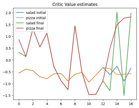
In this we can see that a couple of things

1. For the first 12 tokens the for both salad and pizza predictions are the same, both for initial and trained network. This makes sense because they;re the same tokens

2. After first 12 tokens both the intial and trained networks diverge

3. For the trained network however the value starts rising substantially we get more “pizza” tokens. This is what we’re looking for. Since the reward is given on full ["p", "i", "z", "z" "a"] completion this is estimate of that future value being projected onto earlier states.

Load an earlier checkpoint

We also can load an earlier checkpoint to see what the completions looked liked. In this case it seems were already close getting more pizza completions, but not as many as our final checkpoint.

As an exercise keep training going to see what happens.

filepath = "temp/ppo/pizza/ppo_checkpoint_episode_100.pt"

policy_step_100, _, _, _, _ = load_ppo_checkpoint(filepath)

2025-11-11 19:35:44,409 - INFO - Loaded PPO checkpoint from temp/ppo/pizza/ppo_checkpoint_episode_100.pt, at episode 100

for _ in range(20):
    final_output = policy_step_100.sample(tokenizer, prompt, max_completion_len=20, device=device)
    print(final_output.text)

ravin likes pizzaE
ravin likes pizzaE
ravin likes pizzaE
ravin likes pizzaE
ravin likes pizzaE
ravin likes pizzaE
ravin likes pizzfE
ravin likes pizzaE
ravin likes pizzaE
ravin likes pizzaE
ravin likes nookiesE
ravin likes applesE
ravin likes pizzaE
ravin likes piaPE
ravin likes bE
ravin likes pizzaE
ravin likes bE
ravin likes applesE
ravin likes pizzaE
ravin likes pizzaE

pizza_bool = []
prompt = "ravin likes "

for _ in range(100):
    final_output = policy_step_100.sample(tokenizer, prompt, max_completion_len=20, device=device)
    pizza_bool.append("pizza" in final_output.text)

torch.tensor(pizza_bool, dtype=torch.float).mean()

tensor(0.5100)

Suggested Prompts

• What are the benefits for PPO for LLM training? What are the challenges?

• What are the mathematical considerations for LLM? What about engineering considerations?

• How sensitive are LLMs to RL updates?

References

• OpenAI Spinning Up - PPO explained in early OpenAI with math and older PyTorch notation.

• Clean RL Implementation - A code first implementation of PPO.

• HuggingFace PPO Guide - Another intuitive explanation of PPO with many good graphics.