Audio Tokenization Tutorial

TLDR:
To put our audio tokenization knowledge into practice, we’ll be using Vector Quantization (VQ) to represent audio in a compact, discrete form.

We’ll:

• Convert our audio into a spectrogram.

• Use VQ with K-Means to cluster similar parts of the spectrogram.

• Analyze the tokens generated by VQ.

• Reconstruct the audio from the tokens.

What You Should Be Familiar With

Since this tutorial covers a practical implementation of audio tokenization, you should be familiar with audio tokenization, why it’s useful, Vector Quantization (VQ), and you should be comfortable with the following concepts:

• How to work with audio data in Python

• How to visualize audio signals and create spectrograms.

• The various audio features that can be extracted from audio signals, and how to extract them.

If you’re new to these concepts, we cover all of them in detail in the Audio Features Tutorial. I recommend checking it out before diving into this tutorial.

By the end of this tutorial, you’ll have a solid understanding of how to tokenize audio and the potential applications of this technique. We’ll use VQ to group similar audio features together and represent them with a single token. This helps us create a finite “vocabulary” for our audio, much like how we use a limited set of words to express a vast range of ideas in language.

Let’s get started by setting up our environment and diving into the code!

Setup

Before we dive into the exciting world of audio tokenization, we need to set up our environment. This section will guide you through the process of importing the necessary libraries and preparing our workspace.

Required Libraries

For this tutorial, we’ll be using several Python libraries that are essential for audio processing and machine learning. Let’s import them:

import numpy as np
import librosa 
import soundfile as sf
from sklearn.cluster import KMeans
import matplotlib.pyplot as plt
import IPython.display as ipd

Let’s break down why we need each of these libraries:

• numpy (np): This is our go-to library for numerical operations. We’ll use it for handling arrays and performing various calculations.

• librosa: This is a powerful library specifically designed for music and audio analysis. We’ll use it to load audio files, compute spectrograms, and perform audio signal processing.

• soundfile (sf): This library allows us to read and write sound files. We’ll use it to save our reconstructed audio.

• sklearn.cluster.KMeans: This is the implementation of the K-Means clustering algorithm that we’ll use for Vector Quantization.

• matplotlib.pyplot (plt): This is our plotting library. We’ll use it to visualize our audio signals, spectrograms, and tokenized representations.

• IPython.display (ipd): This will allow us to play audio directly in our Jupyter notebook.

Load Audio and Create Spectrogram

Now that we have our environment set up, let’s start by loading an audio file and converting it into a Mel spectrogram. We’ll use the Mel spectrogram as the input for our Vector Quantization model.

First, we need to define a function for loading and preprocessing audio.

def load_and_preprocess_audio(file_path, sr=None, n_mels=80):
    y, sr = librosa.load(file_path, sr=sr)
    mel_spec = librosa.feature.melspectrogram(y=y, sr=sr, n_mels=n_mels)
    log_mel_spec = librosa.power_to_db(mel_spec)
    return y, sr, log_mel_spec

• It takes a file path, target sampling rate (sr), and number of mel bands (n_mels) as inputs.

• It uses librosa to load the audio file and resample it if necessary.

• It then computes a mel spectrogram, which is a representation of the audio that mimics how human hearing perceives sound frequencies.

• Finally, it converts the spectrogram to a logarithmic scale, which better represents how we perceive loudness.

audio_file = librosa.example('trumpet') # Here I'm using a sample audio file from librosa
# audio_file = "path_to_your_audio_file.wav"  # Replace with your audio file path

y, sr, mel_features  = load_and_preprocess_audio(audio_file)

print(f"Mel spectrogram shape: {mel_features.shape}")
print(f"Sampling rate: {sr}")
print(f"Original audio length: {y.shape[0]} samples")

ipd.Audio(y, rate=sr)

Mel spectrogram shape: (80, 230)
Sampling rate: 22050
Original audio length: 117601 samples

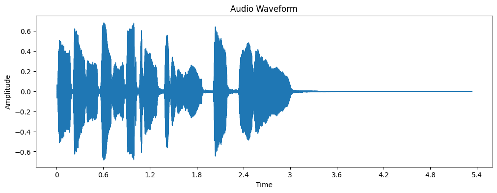
We can visualize the waveform first.

plt.figure(figsize=(12, 4))
librosa.display.waveshow(y, sr=sr)
plt.title('Audio Waveform')
plt.xlabel('Time')
plt.ylabel('Amplitude')
plt.show()

Visualizing the Spectrogram

Now, let’s take a look at the Mel spectrogram we computed.

plt.figure(figsize=(12, 4))
librosa.display.specshow(mel_features, sr=sr, x_axis='time', y_axis='mel')
plt.colorbar(format='%2.0f dB')
plt.title('Mel Spectrogram')
plt.show()

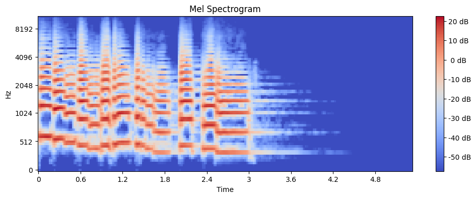
This colorful plot shows the intensity of different frequencies over time. The x-axis represents time, the y-axis represents mel frequency bands, and the color intensity represents the loudness at each time-frequency point.

Why Mel Spectrograms?

You might be wondering why we’re using mel spectrograms instead of raw waveforms. There are a few good reasons:

• Mel spectrograms are more compact representations of audio.

• They emphasize the frequency ranges that humans are more sensitive to.

• Many audio processing tasks (like speech recognition) perform better with spectrograms than raw waveforms.

• In the next section, we’ll use this mel spectrogram as the input for our Vector Quantization process. We’re one step closer to tokenizing our audio!

Vector Quantization (VQ) Tokenization

Now that we have our audio in the form of a mel spectrogram, we’re ready to dive into the heart of our process: tokenization using Vector Quantization (VQ). This is where we transform our continuous audio representation into a discrete, symbolic form.

Understanding Vector Quantization

Before we jump into the code, let’s take a moment to really understand what Vector Quantization is and why it’s so powerful.

Vector Quantization is a classic technique from signal processing that allows us to compress a large set of data points into a smaller set of representative points.

Let’s break it down with an analogy:

Crayons Analogy

Imagine you have a giant box of crayons with thousands of slightly different shades. Vector Quantization is like choosing a smaller set of crayons (let’s say 512) that can best represent all the colors in the original set. Now, for any color in the original set, we’d use the closest color from our smaller set to represent it.

In our audio context:

• The original crayons are all the possible sound fragments in our mel spectrogram.

• Our smaller crayon set is our “codebook” or token vocabulary.

• The process of matching original colors to the smaller set is our tokenization.

Implementing VQ Tokenization

Now, let’s examine our VQ tokenization function in detail:

def vq_tokenize(features, n_tokens=512):
    # Flatten the 2D features to 1D
    flattened_features = features.T.flatten()
    
    # Reshape to 2D array (required input shape for KMeans)
    reshaped_features = flattened_features.reshape(-1, 1)
    
    # Perform K-means clustering
    kmeans = KMeans(n_clusters=n_tokens, random_state=42)
    kmeans.fit(reshaped_features)
    
    # Get cluster assignments (tokens)
    tokens = kmeans.predict(reshaped_features)
    
    # Reshape tokens back to original shape (time, frequency)
    tokens = tokens.reshape(features.shape[1], -1)
    
    return tokens, kmeans

Let’s break this down step by step:

• Flattening: We start by flattening our 2D mel spectrogram into a 1D array. This is because K-means works with 1D vectors.

• Reshaping: We reshape our flattened array into a 2D array where each row is a single data point. This is the required input format for sklearn’s KMeans function.

• K-means Clustering: This is where the actual Vector Quantization happens. K-means is an algorithm that tries to partition our data points into n_tokens clusters. Each cluster will be represented by its centroid, and these centroids become our token vocabulary.

• Token Assignment: Once K-means has found our clusters, we use it to predict which cluster each of our original data points belongs to. This assignment of data points to clusters is our tokenization.

• Reshaping: Finally, we reshape our tokens back into the original shape of our mel spectrogram. This allows us to maintain the time-frequency structure of our audio.

Now, let’s apply this to our mel spectrogram:

n_tokens = 64  # This is our vocabulary size
tokens, kmeans_model = vq_tokenize(mel_features, n_tokens)

print(f"Shape of tokens: {tokens.shape}")
print(f"Number of unique tokens: {len(np.unique(tokens))}")

Shape of tokens: (230, 80)
Number of unique tokens: 64

Visualizing the Tokenized Representation

Visualization can provide great insights into our tokenized audio. Let’s create a color-coded representation:

plt.figure(figsize=(12, 4))
plt.imshow(tokens, aspect='auto', interpolation='nearest', cmap='viridis')
plt.colorbar(label='Token ID')
plt.title('Tokenized Audio')
plt.xlabel('Time')
plt.ylabel('Frequency')
plt.show()

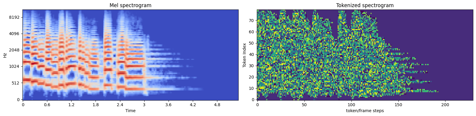
In this plot:

• The x-axis represents time,

• The y-axis represents frequency bands.

• Each color represents a different token.

You might notice patterns in this visualization:

• Vertical stripes often represent sustained sounds.

• Rapid color changes might indicate transient sounds or percussive elements.

• Large blocks of a single color could represent silence or background noise.

Analyzing Token Distribution

Understanding how our tokens are used can provide insights into our audio and the effectiveness of our tokenization:

token_counts = np.bincount(tokens.flatten())
plt.figure(figsize=(12, 4))
plt.bar(range(len(token_counts)), token_counts)
plt.title('Token Frequency Distribution')
plt.xlabel('Token ID')
plt.ylabel('Frequency')
plt.show()

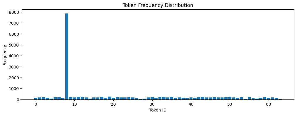
This histogram shows how often each token appears in our audio. Here’s what we can learn from this distribution:

• Are some tokens used much more frequently than others? In the audio example we used, token 8 is the most common.

• Are there tokens that are never or rarely used? This might suggest we could use fewer tokens without losing much information. For example, token 27 is used in our audio only once.

• Is the distribution relatively even? This could indicate a good utilization of our token vocabulary. In our case, token 8 is used much more frequently than others.

# Get the indices of min and max frequency tokens 
min_token_id = np.argmin(token_counts)
max_token_id = np.argmax(token_counts)

print(f"Token ID with minimum frequency: {min_token_id} : {token_counts[min_token_id]}")
print(f"Token ID with maximum frequency: {max_token_id} : {token_counts[max_token_id]}")

Token ID with minimum frequency: 27 : 58
Token ID with maximum frequency: 8 : 7856

Note

Note that this distribution can vary widely depending on the audio content. So, try this with your audio!

At this point, we’ve transformed our continuous audio signal into a sequence of discrete tokens. This transformation is powerful for several reasons:

• Compression: We’ve represented our complex audio using only 512 unique tokens. This can lead to significant data compression.

• Discretization: We’ve moved from a continuous space (amplitude values in the spectrogram) to a discrete space (token IDs). This can make subsequent processing steps easier.

• Semantic Representation: Each token can be thought of as representing a specific “audio concept”. This can be powerful for tasks like audio understanding or generation.

• Machine Learning Friendly: Many machine learning models are designed to work with discrete tokens. Our tokenized audio is now in a format that’s readily usable by such models.

Now that we’ve successfully tokenized our audio, let’s explore the reverse process: converting our tokens back into audio. This process involves two main steps: detokenization (converting tokens back to a mel spectrogram) and audio reconstruction (converting the mel spectrogram back to an audio waveform).

Detokenization

First, let’s implement our detokenization function:

def vq_detokenize(tokens, kmeans):
    # Flatten the tokens
    flattened_tokens = tokens.flatten()
    
    # Use the centroids of the K-means clusters to reconstruct the features
    reconstructed_features = kmeans.cluster_centers_[flattened_tokens]
    
    # Reshape back to the original mel spectrogram shape
    reconstructed_features = reconstructed_features.reshape(tokens.shape[0], tokens.shape[1], -1)
    
    # Remove the unnecessary dimension
    return reconstructed_features.squeeze()

This function does the following:

• Flattens our 2D token array into a 1D array.

• Uses our K-means model to look up the centroid (average feature vector) for each token.

• Reshapes the result back into the original mel spectrogram shape.

Let’s apply this function to our tokens:

reconstructed_mel = vq_detokenize(tokens, kmeans_model)

print(f"Shape of reconstructed mel spectrogram: {reconstructed_mel.shape}")

Shape of reconstructed mel spectrogram: (230, 80)

Comparing Original and Reconstructed Spectrograms

Now, let’s visually compare our original mel spectrogram with the reconstructed one.

fig, (ax1, ax2) = plt.subplots(2, 1, figsize=(12, 8))

img1 = librosa.display.specshow(mel_features, x_axis='time', y_axis='mel', ax=ax1)
ax1.set_title('Original Mel Spectrogram')
fig.colorbar(img1, ax=ax1, format='%2.0f dB')

img2 = librosa.display.specshow(reconstructed_mel.T, x_axis='time', y_axis='mel', ax=ax2)
ax2.set_title('Reconstructed Mel Spectrogram')
fig.colorbar(img2, ax=ax2, format='%2.0f dB')

plt.tight_layout()
plt.show()

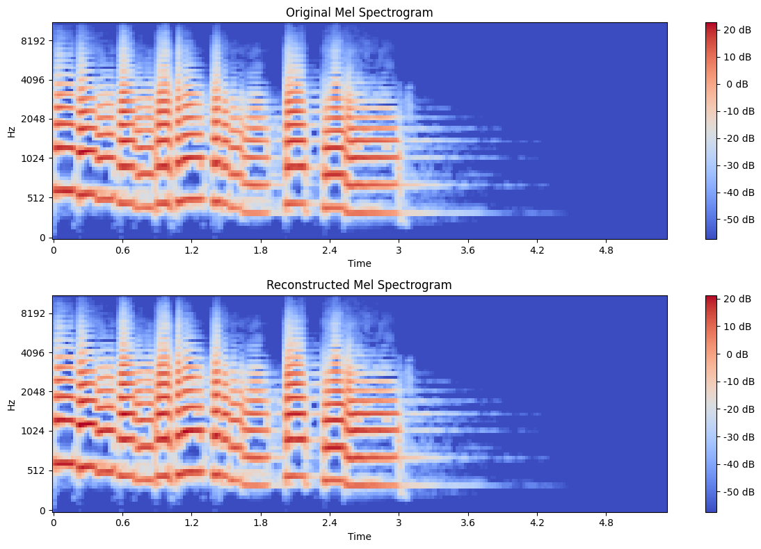
Observe the differences between the two spectrograms. The reconstructed spectrogram looks a bit “blockier” or less detailed. This is because our tokenization process has quantized the continuous spectrogram into a discrete set of values.

Audio Reconstruction

Now, let’s convert our reconstructed mel spectrogram back into an audio waveform. We’ll use the Griffin-Lim algorithm for this purpose:

def mel_to_audio(mel_spec, sr, n_iter=10):
    # Convert from dB scale back to power
    mel_spec = librosa.db_to_power(mel_spec)
    
    # Use librosa's built-in Griffin-Lim implementation
    y_reconstructed = librosa.feature.inverse.mel_to_audio(mel_spec.T, sr=sr, n_iter=n_iter)
    
    return y_reconstructed

# Reconstruct audio
reconstructed_audio = mel_to_audio(reconstructed_mel, sr)

# Trim or pad to match original length
if len(reconstructed_audio) > len(y):
    reconstructed_audio = reconstructed_audio[:len(y)]
else:
    reconstructed_audio = np.pad(reconstructed_audio, (0, len(y) - len(reconstructed_audio)))

The Griffin-Lim algorithm estimates phase information (which was lost during the conversion to mel spectrogram) to reconstruct the audio signal.

Comparing Original and Reconstructed Audio

Let’s listen to both the original and reconstructed audio:

print("Original Audio:")
ipd.display(ipd.Audio(y, rate=sr))

print("Reconstructed Audio:")
ipd.display(ipd.Audio(reconstructed_audio, rate=sr))

Original Audio:

Reconstructed Audio:

You can notice some differences between the original and reconstructed audio. The reconstructed version might sound a bit distorted or warped compared to the original. This is due to several factors:

• Information loss during the mel spectrogram conversion

• Further information loss during tokenization

• Imperfect phase reconstruction by the Griffin-Lim algorithm

Comparing Waveforms

Finally, let’s visually compare the waveforms of the original and reconstructed audio:

fig, (ax1, ax2) = plt.subplots(2, 1, figsize=(12, 8))

librosa.display.waveshow(y, sr=sr, ax=ax1)
ax1.set_title('Original Waveform')

librosa.display.waveshow(reconstructed_audio, sr=sr, ax=ax2)
ax2.set_title('Reconstructed Waveform')

plt.tight_layout()
plt.show()

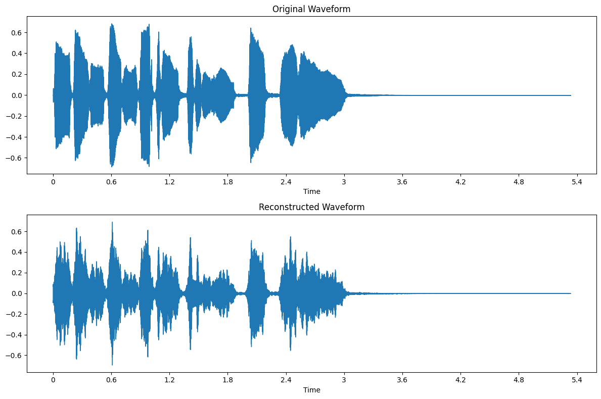
Observe how the general structure of the waveform is preserved, but fine details may be lost, leading to differences in sound quality.

Section Summary

This reconstruction process demonstrates both the power and limitations of our tokenization approach:

• Compression: We’ve represented our audio using a small set of tokens, achieving significant compression.

• Information Preservation: The reconstructed audio maintains much of the structure of the original, showing that our tokens capture essential audio characteristics.

• Quality Trade-off: There’s a noticeable loss in audio quality, highlighting the trade-off between compression and fidelity.

In the next section, we’ll explore ways to adjust our tokenization process to balance these factors and potentially improve our results.

Experimenting with Parameters

Our tokenization process involves several parameters that we can adjust to potentially improve our results. Let’s experiment with some of these:

Number of Tokens

We can try different numbers of tokens to see how it affects our audio quality and compression:

for n_tokens in [8, 32, 64, 128, 256]:
    tokens, kmeans_model = vq_tokenize(mel_features, n_tokens)
    reconstructed_mel = vq_detokenize(tokens, kmeans_model)
    reconstructed_audio = mel_to_audio(reconstructed_mel, sr)
    
    print(f"\nNumber of tokens: {n_tokens}")
    print(f"Compression ratio: {mel_features.size / tokens.size:.2f}x")
    
    ipd.display(ipd.Audio(reconstructed_audio, rate=sr))

Number of tokens: 8
Compression ratio: 1.00x

Number of tokens: 32
Compression ratio: 1.00x

Number of tokens: 64
Compression ratio: 1.00x

Number of tokens: 128
Compression ratio: 1.00x

Number of tokens: 256
Compression ratio: 1.00x

Listen to the audio for each number of tokens. How does the audio quality change? At what point do you stop hearing improvements?

Mel Spectrogram Parameters

We can also adjust parameters of our mel spectrogram:

for n_mels in [2, 20, 40, 80, 160]:
    _, _, log_mel_spec = load_and_preprocess_audio(audio_file, sr=sr, n_mels=n_mels)
    tokens, kmeans_model = vq_tokenize(mel_features, n_tokens=64)
    reconstructed_mel = vq_detokenize(tokens, kmeans_model)
    reconstructed_audio = mel_to_audio(reconstructed_mel, sr)
    
    print(f"\nNumber of mel bands: {n_mels}")
    ipd.display(ipd.Audio(reconstructed_audio, rate=sr))

Number of mel bands: 2

Number of mel bands: 20

Number of mel bands: 40

Number of mel bands: 80

Number of mel bands: 160

How does changing the number of mel bands affect the audio quality? Try with your audio files and see how these parameters impact the results.

Potential Optimizations

There are several ways we might further improve our tokenization process:

• Advanced Clustering: We used K-means for simplicity, but more advanced clustering algorithms like Gaussian Mixture Models might yield better results.

• Perceptual Weighting: We could weight our feature vectors based on human auditory perception, potentially improving the perceptual quality of our reconstructed audio.

• Context-Aware Tokenization: Instead of tokenizing each time-frequency bin independently, we could consider local context, potentially capturing more temporal structure.

• Neural Approaches: Deep learning models like VQ-VAE (Vector Quantized Variational Autoencoder) have shown promising results in audio tokenization tasks.

Conclusion

In this tutorial, we’ve explored the process of audio tokenization using Vector Quantization. We’ve seen how we can represent complex audio signals using a discrete set of tokens, and how we can reconstruct audio from these tokens.

Key takeaways:

• Audio can be effectively represented and compressed using discrete tokens.

• There’s a trade-off between compression (fewer tokens) and audio quality.

• The process involves several steps (mel spectrogram conversion, tokenization, detokenization, audio reconstruction), each with its own challenges and opportunities for optimization.

• While our reconstructed audio isn’t perfect, it maintains much of the structure and content of the original, demonstrating the power of this approach.

As we’ve seen, audio tokenization opens up exciting possibilities in various areas of audio processing and machine learning. While our implementation is relatively simple, it provides a foundation for understanding more advanced techniques in this field.

Continue experimenting with this code, try out some of the suggested optimizations, and explore how you might apply audio tokenization in your own projects!

References

• Chapter 7 of Speech Coding With Code-Excited Linear Prediction by Tom Bäckström. This book provides a comprehensive overview of Vector Quantization and its applications in speech coding and compression.

• K-Means Clustering in Python - Official documentation for the K-Means clustering algorithm in scikit-learn.