Audio Features

TLDR:

• Audio features are measurable properties of audio signals that can be used to describe and analyze sound.

• Features capture different aspects of audio:

  • Temporal

  • Spectral

  • Perceptual

  • Musical.

• Extracted features can be used for various tasks like:

  • Classification

  • Recognition

  • Tokenization

  • Generation

• We’ll Cover in this Tutorial:

  • Loading and visualizing audio files

  • Time-domain features:

    • RMS Energy

    • Zero Crossing Rate

  • Frequency-domain features:

    • STFT

    • Spectral Centroid

    • Spectral Rolloff

  • Mel-frequency Cepstral Coefficients (MFCCs)

  • Chroma Features (for musical analysis)

By the end of this tutorial, you’ll understand how to extract and interpret various audio features using Python and librosa.

Setting the Stage

Imagine you’re a music enthusiast with a vast collection of songs. You can easily distinguish between different genres, identify instruments, or even recognize specific artists just by listening. But how can we teach a computer to do the same? This is where audio feature extraction comes in.

To train a statistical or machine learning model to understand audio, we need to present the audio data in a format that the model can process. This is like teaching a computer to “hear” music or sound the way we do.

Audio feature extraction is a necessary step in any audio related task, and it describes the process of analyzing audio signals to extract meaningful information that can be used for various applications. Think of it as breaking down the complex world of sound into simpler, measurable components.

What are the the different types of audio features?

Audio features can be broadly categorized into several types. Let’s break them down:

• Time-domain features: These features are extracted directly from the waveform of the audio signal.

  Imagine you’re looking at a river. The height of the waves (amplitude) and how often they come (frequency) can tell you a lot about the river’s flow. Similarly, time-domain features like Amplitude Envelope, Root Mean Square (RMS) Energy, and Zero-crossing rate (zcr) give us information about the audio signal’s behavior over time.

• Frequency-domain features: These features are derived from the frequency representation of the audio signal.

  Picture a choir with different voice types - bass, tenor, alto, and soprano. Each voice type occupies a different frequency range. Frequency-domain features help us understand which “voices” or frequencies are present in our audio and how strong they are. Examples include:

  • Spectral Centroid

  • Spectral Rolloff

  • Spectral Flux

  • Spectral Bandwidth.

• Time-frequency domain features: These features represent both time and frequency characteristics of the audio.

  Imagine you’re watching a movie in slow motion. You can see how the scene changes over time and how different colors (frequencies) appear and disappear. Time-frequency domain features like Short-time Fourier Transform (STFT), Mel-frequency Cepstral Coefficients (MFCCs), and Constant-Q Transform capture this dynamic relationship between time and frequency.

Before we dive into the details of audio features and how to extract them, we need to learn how to deal with audio data. In the next section, we’ll explore the basics of audio data representation and how to load and visualize audio files in Python.

# Import necessary libraries
import numpy as np # Numerical computing and array operations
import librosa # Audio and music processin
import librosa.display # Data visualization
import matplotlib.pyplot as plt
import IPython.display as ipd # Interactive display of audio in Jupyter notebooks
from scipy.io import wavfile # Audio file I/O operations
import pandas as pd # Data manipulation and analysis

Now that we have our libraries imported and a comprehensive understanding of audio feature extraction, let’s proceed to load and visualize an audio file in the next section.

Loading and Visualizing Audio Files

Understanding audio data is crucial before we dive into feature extraction. In this section, we’ll explore how to load audio files, examine their properties, and visualize them in various ways. This process helps us gain insights into the audio signal’s characteristics and prepares us for feature extraction.

# Load an audio file
audio_path = librosa.example('trumpet') # You can use a sample audio file from librosa
# audio_path = "path/to/your/audio/file.wav" # Or replace with your audio file
y, sr = librosa.load(audio_path)

Downloading file 'sorohanro_-_solo-trumpet-06.ogg' from 'https://librosa.org/data/audio/sorohanro_-_solo-trumpet-06.ogg' to '/home/fadi2/.cache/librosa'.

Let’s break down what’s happening here:

• librosa.load() reads the audio file and returns two variables:

  • y: The audio time series as a numpy array

  • sr: The sampling rate of the audio

By default, librosa resamples the audio to 22050 Hz. You can specify a different sampling rate or use the native sampling rate of the file by setting sr=None.

Understanding Audio Properties

Now that we’ve loaded our audio file, let’s examine its basic properties.

# Display basic information about the audio file
duration = librosa.get_duration(y=y, sr=sr)
print(f"Audio duration: {duration:.2f} seconds")
print(f"Sample rate: {sr} Hz")
print(f"Number of samples: {len(y)}")
print(f"Shape of audio array: {y.shape}")

Audio duration: 5.33 seconds
Sample rate: 22050 Hz
Number of samples: 117601
Shape of audio array: (117601,)

These properties tell us:

• Duration: The length of the audio in seconds

• Sample rate: The number of samples per second (typically 22050 Hz for librosa)

• Number of samples: Total data points in the audio signal

• Shape: The dimensions of the numpy array (should be 1D for mono audio)

Playing the Audio

It’s often helpful to listen to the audio we’re analyzing. In Jupyter notebooks, we can use IPython.display.Audio to play the audio directly in the notebook.

# Play the audio file
ipd.display(ipd.Audio(y, rate=sr))

Visualizing the Waveform

The waveform is a basic visual representation of the audio signal. It shows the amplitude of the signal over time.

# Visualize the waveform
plt.figure(figsize=(14, 5))
librosa.display.waveshow(y, sr=sr)
plt.title("Audio Waveform")
plt.xlabel("Time")
plt.ylabel("Amplitude")
plt.show()

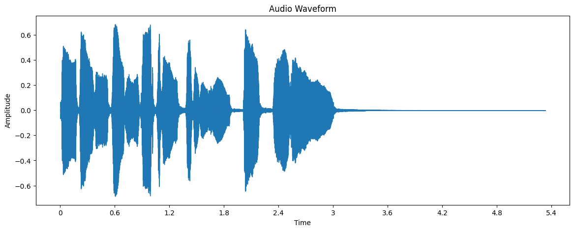
Here’s how to interpret the waveform:

• The x-axis represents time

• The y-axis represents the amplitude of the signal

• Louder parts of the audio will have larger amplitudes (taller waves)

• Quiet parts will be closer to the center line

Visualizing the Spectrogram

While the waveform shows amplitude over time, a spectrogram shows how the frequency content of the signal changes over time. It’s a 2D representation with time on the x-axis, frequency on the y-axis, and color representing the intensity of each frequency at each time point.

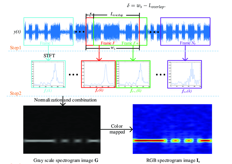
Fig. 43 name: stft-flowchart Short-Time Fourier Transform (STFT) Flowchart source

To compute the spectrogram, we use the Short-Time Fourier Transform (STFT). The STFT breaks the audio signal into short overlapping frames and computes the Fourier Transform for each frame. This gives us a time-varying representation of the frequency content of the audio.

# Compute the spectrogram
D = librosa.stft(y)  # STFT of y
S_db = librosa.amplitude_to_db(np.abs(D), ref=np.max)  # Convert to dB scale

# Display the spectrogram
plt.figure(figsize=(14, 5))
librosa.display.specshow(S_db, sr=sr, x_axis='time', y_axis='hz')
plt.colorbar(format='%+2.0f dB')
plt.title('Spectrogram')
plt.show()

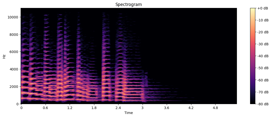
Here’s how to interpret the spectrogram:

• The x-axis represents time

• The y-axis represents frequency

• The color intensity represents the amplitude of each frequency at each time point

• Brighter colors indicate higher amplitudes

• This visualization helps identify dominant frequencies, harmonics, and how the frequency content changes over time

Visualizing Mel Spectrogram

A Mel spectrogram is similar to a regular spectrogram, but the frequency scale is converted to the Mel scale, which better represents human auditory perception.

# Compute the mel spectrogram
S = librosa.feature.melspectrogram(y=y, sr=sr, n_mels=128)
S_db_mel = librosa.power_to_db(S, ref=np.max)

# Display the mel spectrogram
plt.figure(figsize=(14, 5))
librosa.display.specshow(S_db_mel, sr=sr, x_axis='time', y_axis='mel')
plt.colorbar(format='%+2.0f dB')
plt.title('Mel Spectrogram')
plt.show()

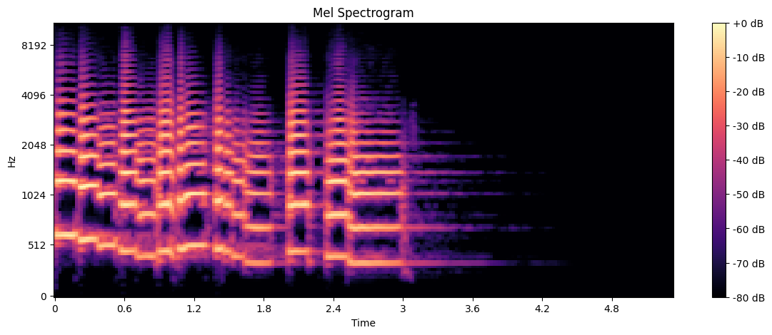
The Mel spectrogram:

• Provides a representation that’s closer to how humans perceive sound

• Often used as input for machine learning models in audio classification tasks

Section Summary

In this section, we learned how to:

• Load audio files using librosa

• Examine basic audio properties

• Play audio in a Jupyter notebook

• Visualize audio as a waveform

• Create and interpret spectrograms and mel spectrograms

Time-domain Features

Time-domain features are extracted directly from the audio waveform. These features capture temporal characteristics of the audio signal and are often computationally efficient to calculate. In this section, we’ll explore two important time-domain features: Root Mean Square (RMS) Energy and Zero Crossing Rate (ZCR).

Root Mean Square (RMS) Energy

RMS Energy is a measure of the signal’s overall energy or loudness over time. It provides insight into the amplitude variations of the audio signal.

Mathematical definition:

\[RMS = \sqrt{\frac{1}{N} \sum_{i=1}^{N} x_i^2}\]

where \(x_i\) are the sample values and \(N\) is the number of samples in the frame.

Let’s calculate and visualize the RMS energy:

# Calculate RMS energy
frame_length = 2048
hop_length = 512
rms = librosa.feature.rms(y=y, frame_length=frame_length, hop_length=hop_length)

# Plot RMS energy
plt.figure(figsize=(14, 5))
times = librosa.times_like(rms, sr=sr, hop_length=hop_length)
plt.plot(times, rms[0])
plt.title("Root Mean Square Energy")
plt.xlabel("Time (seconds)")
plt.ylabel("RMS Energy")
plt.show()

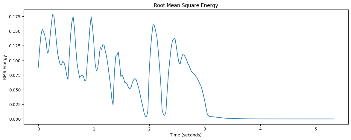
Here’s how to interpret the RMS Energy plot:

• The x-axis represents time in seconds.

• The y-axis represents the RMS energy.

• Higher values indicate louder segments of the audio.

• Lower values indicate quieter segments.

RMS Energy is a useful feature for many audio analysis tasks, such as:

• Detecting silence or pauses in speech

• Identifying loud sections in music for beat detection

• Audio segmentation based on energy levels

• Voice activity detection in speech processing

Zero Crossing Rate (ZCR)

Zero Crossing Rate is the rate at which the signal changes from positive to negative or vice versa. It provides information about the frequency content of the signal and is particularly useful for distinguishing percussive sounds from harmonic sounds in music and consonants from vowels in speech.

Mathematical definition:

\[ZCR = \frac{1}{N-1} \sum_{i=1}^{N-1} \frac{\left| \text{sign}(x[i]) - \text{sign}(x[i-1]) \right|}{2}\]

where \(x[i]\) is the signal at sample \(i\), and \(N\) is the total number of samples.

Let’s calculate and visualize the Zero Crossing Rate:

# Calculate Zero Crossing Rate
zcr = librosa.feature.zero_crossing_rate(y, frame_length=frame_length, hop_length=hop_length)

# Plot Zero Crossing Rate
plt.figure(figsize=(14, 5))
times = librosa.times_like(zcr, sr=sr, hop_length=hop_length)
plt.plot(times, zcr[0])
plt.title("Zero Crossing Rate")
plt.xlabel("Time (seconds)")
plt.ylabel("Zero Crossing Rate")
plt.show()

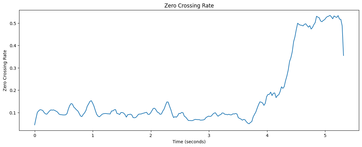
To interpret the ZCR plot:

• The x-axis represents time in seconds.

• The y-axis represents the Zero Crossing Rate.

• Higher values indicate more frequent sign changes, typically associated with higher frequencies or noise.

• Lower values suggest lower frequencies or more tonal sounds.

Applications of Zero Crossing Rate:

• Speech/music discrimination

• Voice activity detection

• Musical genre classification

• Onset detection in music analysis

Combining RMS Energy and Zero Crossing Rate

Often, it’s insightful to view these features together. This allows us to see how the energy and frequency characteristics of the audio signal relate to each other and the original waveform.

Let’s create a combined plot:

plt.figure(figsize=(14, 8))

plt.subplot(2, 1, 1)
librosa.display.waveshow(y, sr=sr, alpha=0.5)
plt.plot(times, rms[0] / rms.max(), color='r', label='RMS Energy')
plt.title("Waveform and RMS Energy")
plt.legend()

plt.subplot(2, 1, 2)
librosa.display.waveshow(y, sr=sr, alpha=0.5)
plt.plot(times, zcr[0], color='g', label='Zero Crossing Rate')
plt.title("Waveform and Zero Crossing Rate")
plt.legend()

plt.tight_layout()
plt.show()

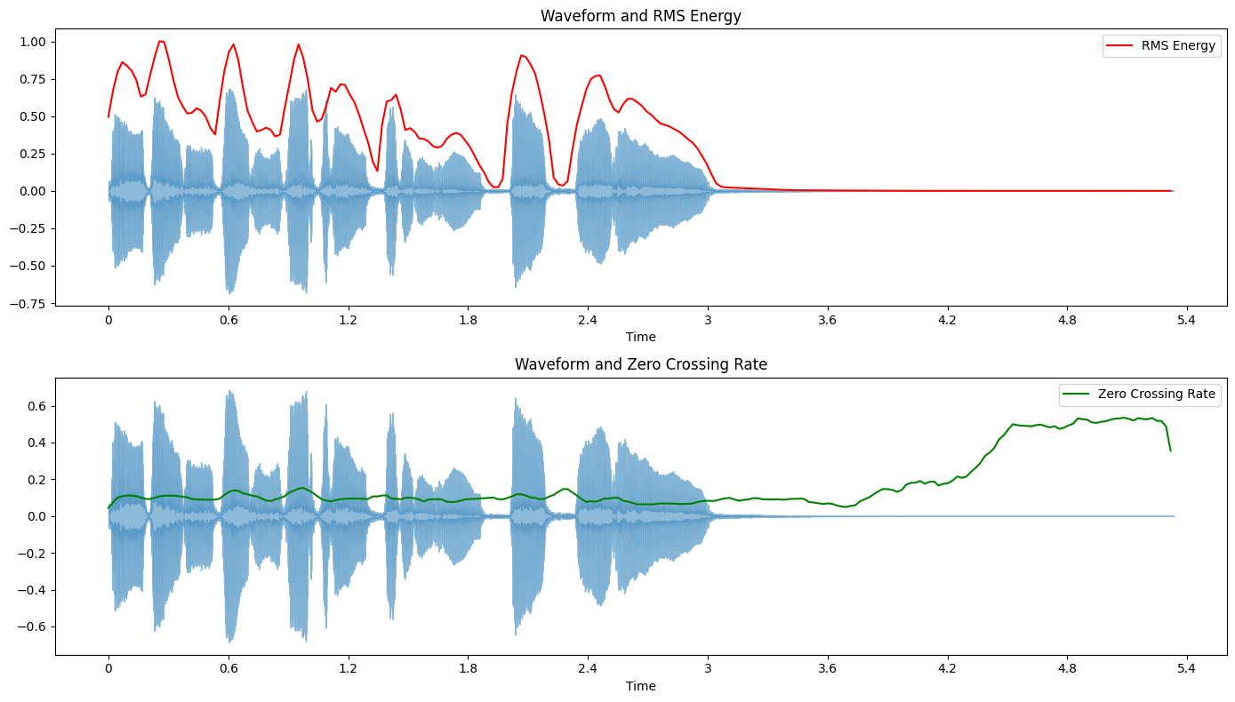
This combined visualization allows us to see how RMS Energy and Zero Crossing Rate relate to the original waveform and to each other.

Feature Statistics

While the time-series of these features is informative, we often need to summarize them for use in machine learning models. Let’s calculate some basic statistics:

# Calculate statistics
rms_mean = np.mean(rms)
rms_std = np.std(rms)
zcr_mean = np.mean(zcr)
zcr_std = np.std(zcr)

print(f"RMS Energy - Mean: {rms_mean:.4f}, Std Dev: {rms_std:.4f}")
print(f"Zero Crossing Rate - Mean: {zcr_mean:.4f}, Std Dev: {zcr_std:.4f}")

RMS Energy - Mean: 0.0529, Std Dev: 0.0553
Zero Crossing Rate - Mean: 0.1735, Std Dev: 0.1522

Section Summary

In this section, we’ve explored two fundamental time-domain features:

• Root Mean Square (RMS) Energy: A measure of the signal’s loudness over time.

• Zero Crossing Rate (ZCR): A measure of the frequency of sign changes in the signal.

These features provide valuable information about the audio signal’s temporal characteristics and are often used as part of a larger feature set for various audio analysis tasks. They are computationally efficient and can be particularly useful for real-time applications.

We learned how to calculate, visualize, and summarize these time-domain features.

In the next sections, we’ll explore frequency-domain features, which will provide different insights into the spectral characteristics of our audio signal.

Frequency-domain Features

While time-domain features give us insights into the temporal characteristics of audio signals, frequency-domain features provide information about the spectral content of the signal. These features are often more informative for tasks like music analysis, genre classification, and speech recognition.

In this section, we’ll explore three important frequency-domain features:

• Short-time Fourier Transform (STFT)

• Spectral Centroid

• Spectral Rolloff

Short-time Fourier Transform (STFT)

The Short-time Fourier Transform (STFT) is a fundamental tool in audio signal processing. It allows us to analyze how frequency content changes over time by applying the Fourier transform to small, overlapping segments of the signal.

Let’s compute and visualize the STFT:

# Compute STFT
n_fft = 2048
hop_length = 512
D = librosa.stft(y, n_fft=n_fft, hop_length=hop_length)

# Convert to dB scale
D_db = librosa.amplitude_to_db(np.abs(D), ref=np.max)

# Visualize the spectrogram
plt.figure(figsize=(14, 6))
librosa.display.specshow(D_db, sr=sr, x_axis='time', y_axis='hz', hop_length=hop_length)
plt.colorbar(format='%+2.0f dB')
plt.title('Short-time Fourier Transform (STFT)')
plt.show()

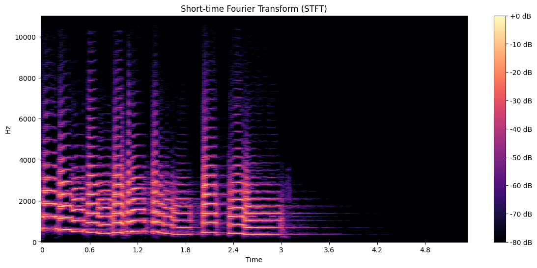
Here’s how to interpret the STFT spectrogram:

• The x-axis represents time.

• The y-axis represents frequency.

• The color intensity represents the magnitude of each frequency component at each time point.

• Brighter colors indicate stronger presence of a frequency at a given time.

STFT is a versatile tool with many applications, including:

• Identifying dominant frequencies in different parts of the audio

• Analyzing harmonic structure in music

• Detecting pitch changes over time

• Serving as a basis for many other audio features and processing techniques

Spectral Centroid

The spectral centroid is a measure of the “center of mass” of the spectrum. It indicates where the “center” of the sound is in terms of frequency. Perceptually, it has a robust connection with the impression of “brightness” of a sound.

Mathematical definition:

\[\text{Spectral Centroid} = \frac{\sum (f \cdot m(f))}{\sum m(f)}\]

where \(f\) is the frequency and \(m(f)\) is the magnitude of the spectrum at that frequency.

Let’s compute and visualize the spectral centroid:

# Compute spectral centroid
centroid = librosa.feature.spectral_centroid(y=y, sr=sr, hop_length=hop_length)

# Visualize spectral centroid
plt.figure(figsize=(14, 6))
times = librosa.times_like(centroid, sr=sr, hop_length=hop_length)
plt.semilogy(times, centroid[0], label='Spectral Centroid')
plt.ylabel('Hz')
plt.xlabel('Time')
plt.legend()
plt.title('Spectral Centroid')
plt.show()

How to interpret the Spectral Centroid plot:

• The x-axis represents time.

• The y-axis represents frequency (in Hz) on a logarithmic scale.

• Higher values indicate a “brighter” sound with more high-frequency content.

• Lower values indicate a “darker” sound with more low-frequency content.

Applications of Spectral Centroid:

• Timbral analysis in music

• Instrument classification

• Audio equalization and filtering

• Voice quality assessment in speech analysis

Spectral Rolloff

Spectral rolloff is the frequency below which a certain percentage (usually 85% or 95%) of the total spectral energy lies. It’s another measure of the spectral shape of the sound.

Let’s compute and visualize the spectral rolloff:

# Compute spectral rolloff
rolloff = librosa.feature.spectral_rolloff(y=y, sr=sr, hop_length=hop_length)

# Visualize spectral rolloff
plt.figure(figsize=(14, 6))
times = librosa.times_like(rolloff, sr=sr, hop_length=hop_length)
plt.semilogy(times, rolloff[0], label='Spectral Rolloff')
plt.ylabel('Hz')
plt.xlabel('Time')
plt.legend()
plt.title('Spectral Rolloff')
plt.show()

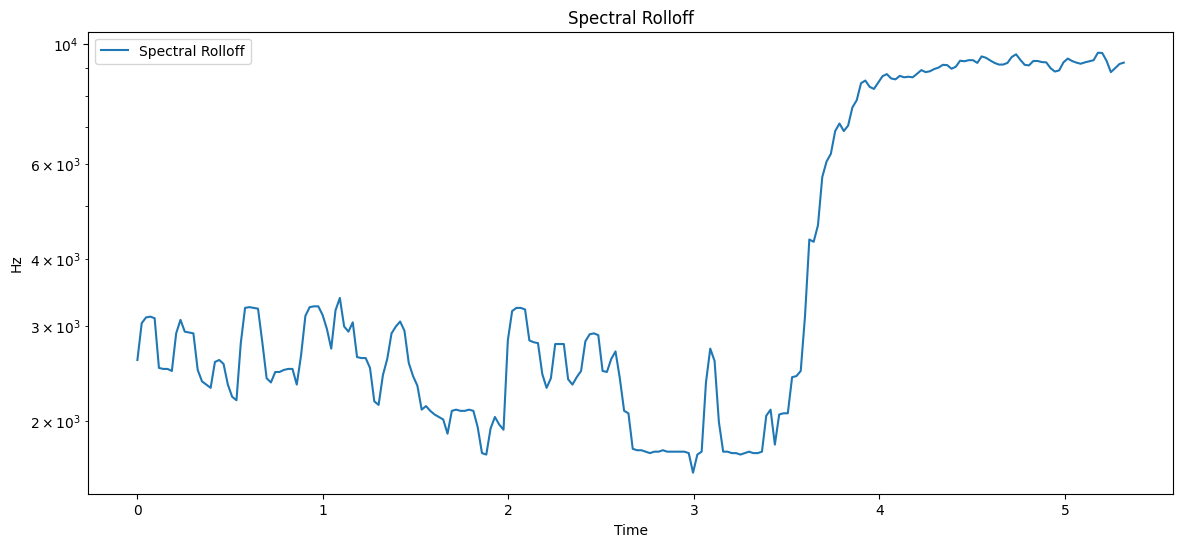
Here’s how to interpret the Spectral Rolloff plot:

• The x-axis represents time.

• The y-axis represents frequency (in Hz) on a logarithmic scale.

• The line shows the frequency below which 85% (by default) of the spectral energy is contained at each time point.

• Higher values indicate more high-frequency content.

Some applications of Spectral Rolloff include:

• Distinguishing between voiced and unvoiced speech

• Music genre classification

• Audio segmentation

• Detecting abrupt spectral changes in audio

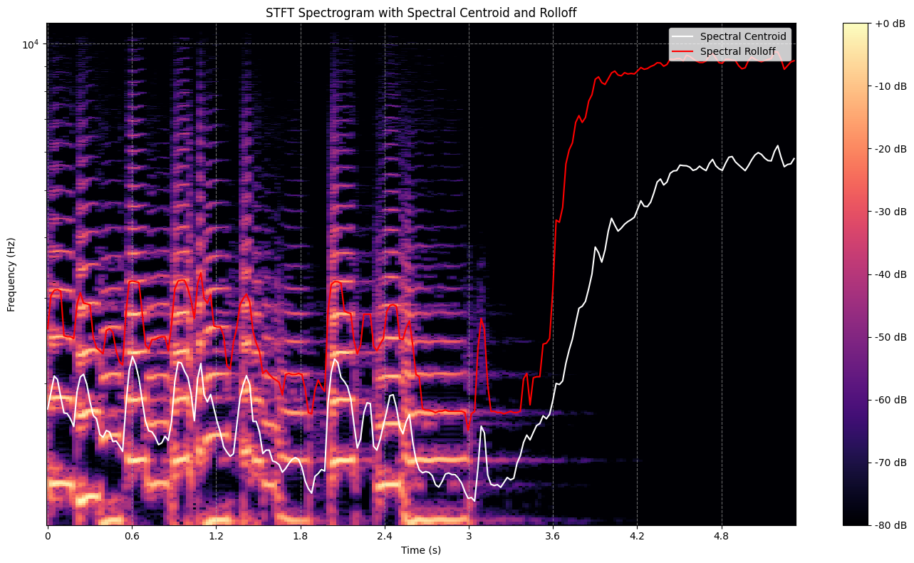
Combining Frequency-domain Features

To get a comprehensive view of the spectral characteristics, let’s visualize these features together:

plt.figure(figsize=(14, 8))

# Plot spectrogram
librosa.display.specshow(D_db, sr=sr, x_axis='time', y_axis='log', hop_length=hop_length)
plt.colorbar(format='%+2.0f dB')
plt.title('STFT Spectrogram with Spectral Centroid and Rolloff')

# Plot spectral centroid on top of the spectrogram
plt.semilogy(times, centroid[0], label='Spectral Centroid', color='w')

# Plot spectral rolloff on top of the spectrogram
plt.semilogy(times, rolloff[0], label='Spectral Rolloff', color='r')

plt.ylabel('Frequency (Hz)')
plt.xlabel('Time (s)')
plt.legend(loc='upper right')
plt.grid(True, linestyle='--', alpha=0.6)
plt.tight_layout()
plt.show()

Feature Statistics

As with time-domain features, it’s often useful to compute summary statistics of these frequency-domain features for use in machine learning models:

# Calculate statistics
centroid_mean = np.mean(centroid)
centroid_std = np.std(centroid)
rolloff_mean = np.mean(rolloff)
rolloff_std = np.std(rolloff)

print(f"Spectral Centroid - Mean: {centroid_mean:.2f} Hz, Std Dev: {centroid_std:.2f} Hz")
print(f"Spectral Rolloff - Mean: {rolloff_mean:.2f} Hz, Std Dev: {rolloff_std:.2f} Hz")

Spectral Centroid - Mean: 2638.40 Hz, Std Dev: 1642.81 Hz
Spectral Rolloff - Mean: 4410.98 Hz, Std Dev: 2993.84 Hz

Section Summary

In this section, we’ve explored three important frequency-domain features:

• Short-time Fourier Transform (STFT): A fundamental tool for analyzing frequency content over time.

• Spectral Centroid: A measure of the “brightness” of a sound.

• Spectral Rolloff: A measure of the shape of the spectrum.

These features provide valuable information about the spectral characteristics of the audio signal and are widely used in various audio analysis tasks. They complement the time-domain features we explored earlier, offering a more complete description of the audio signal.

In the next sections, we’ll delve into more advanced audio features that build upon these fundamental concepts.

Mel-frequency Cepstral Coefficients (MFCCs)

Mel-frequency Cepstral Coefficients (MFCCs) are one of the most widely used features in speech and audio processing. They provide a compact representation of the spectral envelope of a sound that closely relates to how humans perceive pitch and frequency content.

Think of MFCCs as a sound “fingerprint”. Just as your fingerprint is unique to you, MFCCs capture the unique aspects of a sound that help distinguish it from others.

Understanding MFCCs

MFCCs are derived from the following process:

• Take the Fourier transform of a signal

• Map the powers of the spectrum onto the mel scale

• Take the logs of the powers at each of the mel frequencies

• Take the discrete cosine transform of the list of mel log powers

• The MFCCs are the amplitudes of the resulting spectrum

Key concepts:

• Mel scale: A perceptual scale of pitches judged by listeners to be equal in distance from one another

• Cepstrum: The result of taking the Inverse Fourier transform (IFT) of the logarithm of the estimated spectrum of a signal

Let’s compute and visualize the MFCCs:

# Compute MFCCs
n_mfcc = 13
mfccs = librosa.feature.mfcc(y=y, sr=sr, n_mfcc=n_mfcc)

# Visualize MFCCs
plt.figure(figsize=(14, 6))
librosa.display.specshow(mfccs, sr=sr, x_axis='time')
plt.colorbar(format='%+2.0f dB')
plt.title('Mel-frequency Cepstral Coefficients (MFCCs)')
plt.show()

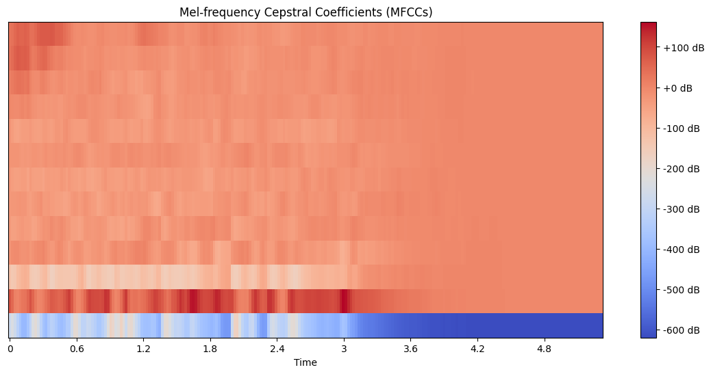
How to interpret the MFCC plot:

• The x-axis represents time.

• The y-axis represents the MFCC coefficients (usually 13, including the 0th coefficient).

• The color intensity represents the magnitude of each coefficient at each time point.

• The lower coefficients (bottom of the plot) represent the overall spectral envelope, while higher coefficients represent finer spectral details.

Analyzing Individual MFCCs

Let’s look at how individual MFCC coefficients change over time:

plt.figure(figsize=(14, 8))
for i in range(4):  # Plot first 4 MFCCs
    plt.subplot(4, 1, i+1)
    plt.plot(librosa.times_like(mfccs), mfccs[i])
    plt.title(f'MFCC {i+1}')
    plt.xlabel('Time')
    plt.ylabel('Magnitude')
plt.tight_layout()
plt.show()

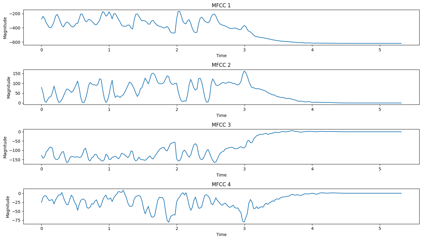
Observations:

• MFCC 1 often correlates with overall energy in the signal.

• Higher-order MFCCs represent increasingly fine spectral details.

• The variations in these coefficients over time capture changes in the spectral characteristics of the audio.

Delta and Delta-Delta MFCCs

In addition to the static MFCC values, it’s often useful to compute their first and second temporal derivatives, known as delta and delta-delta (or acceleration) coefficients. These capture how the MFCCs change over time.

# Compute delta and delta-delta MFCCs
mfccs_delta = librosa.feature.delta(mfccs)
mfccs_delta2 = librosa.feature.delta(mfccs, order=2)

# Visualize delta MFCCs
plt.figure(figsize=(14, 6))
librosa.display.specshow(mfccs_delta, sr=sr, x_axis='time')
plt.colorbar(format='%+2.0f')
plt.title('Delta MFCCs')
plt.show()

# Visualize delta-delta MFCCs
plt.figure(figsize=(14, 6))
librosa.display.specshow(mfccs_delta2, sr=sr, x_axis='time')
plt.colorbar(format='%+2.0f')
plt.title('Delta-Delta MFCCs')
plt.show()

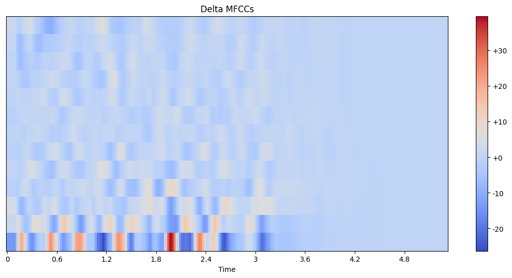
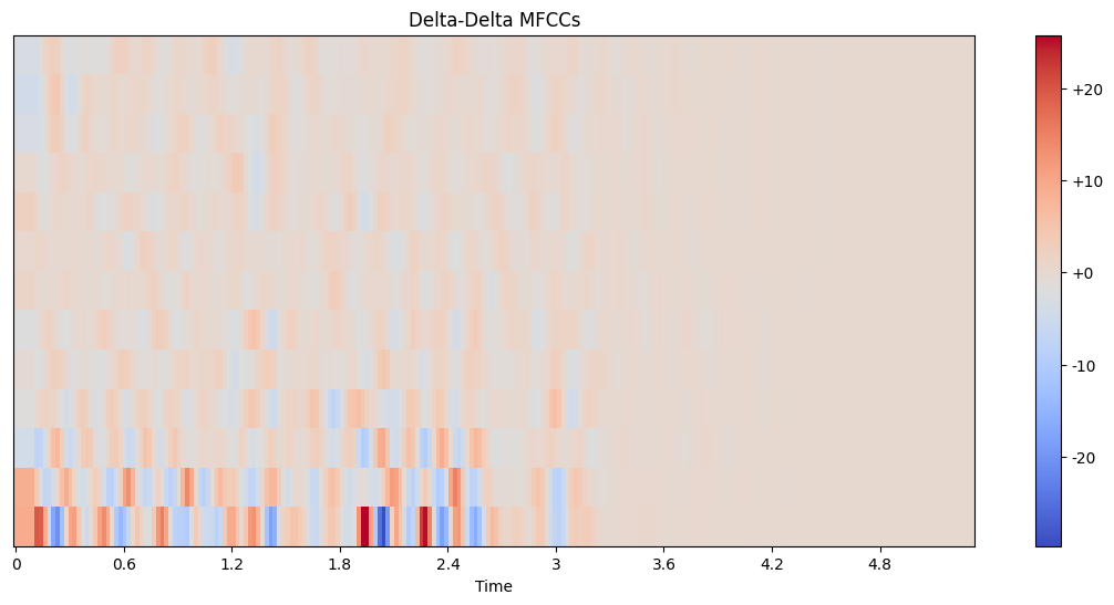
Interpreting delta and delta-delta MFCCs:

• Delta MFCCs represent the rate of change of the MFCC coefficients over time.

• Delta-delta MFCCs represent the acceleration of the MFCC coefficients.

• These features capture dynamic aspects of the audio that static MFCCs might miss.

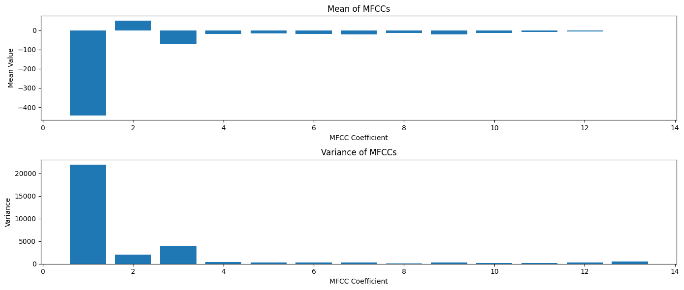
MFCC Statistics

For machine learning applications, we often need to summarize these time-varying features. Let’s compute some basic statistics:

# Calculate statistics
mfcc_means = np.mean(mfccs, axis=1)
mfcc_vars = np.var(mfccs, axis=1)
delta_means = np.mean(mfccs_delta, axis=1)
delta_vars = np.var(mfccs_delta, axis=1)

# Display statistics
plt.figure(figsize=(14, 6))
plt.subplot(2, 1, 1)
plt.bar(range(1, n_mfcc + 1), mfcc_means)
plt.title('Mean of MFCCs')
plt.xlabel('MFCC Coefficient')
plt.ylabel('Mean Value')

plt.subplot(2, 1, 2)
plt.bar(range(1, n_mfcc + 1), mfcc_vars)
plt.title('Variance of MFCCs')
plt.xlabel('MFCC Coefficient')
plt.ylabel('Variance')

plt.tight_layout()
plt.show()

Applications of MFCCs

MFCCs are widely used in various audio processing tasks, including:

• Speech Recognition: MFCCs capture the important characteristics of speech signals.

• Speaker Identification: The spectral shape captured by MFCCs can help distinguish between speakers.

• Music Genre Classification: MFCCs provide a compact representation of timbre, useful for genre analysis.

• Audio Similarity Measurement: MFCCs can be used to compute similarity between audio segments.

• Emotion Recognition in Speech: The spectral characteristics captured by MFCCs correlate with emotional content.

• Audio Tokenization: MFCCs are often used as input features for audio tokenization and compression, these features are used to represent audio segments as tokens.

Limitations of MFCCs

While MFCCs are powerful, they have some limitations:

• They discard phase information, which can be important for some applications.

• They may not capture all relevant information for music analysis, as they were originally designed for speech.

• They can be sensitive to background noise.

Despite these limitations, MFCCs remain a popular choice for many audio processing tasks due to their effectiveness in capturing the spectral characteristics of audio signals.

Section Summary

• Mel-frequency Cepstral Coefficients (MFCCs) provide a compact and perceptually relevant representation of audio signals.

• They capture the spectral envelope of the sound in a way that relates to human auditory perception.

• Along with their delta and delta-delta variants, MFCCs form a powerful set of features for various audio analysis tasks.

• If you want to dive even deeper into MFCCs, here’s a great video: MFCC Explained Easily

In this section, we’ve learned how to:

• Compute and visualize MFCCs

• Analyze individual MFCC coefficients

• Compute delta and delta-delta MFCCs

• Summarize MFCCs using basic statistics

In the next section, we’ll explore chroma features, which are particularly useful for analyzing the harmonic and tonal content of music.

Chroma Features

Chroma features, also known as Pitch Class Profiles, are powerful tools for analyzing the harmonic and tonal content of music. They are particularly useful for tasks involving pitch and harmony analysis, such as chord recognition, key detection, and music similarity estimation.

Understanding Chroma Features

Chroma features represent the intensity of each of the 12 pitch classes (C, C#, D, D#, E, F, F#, G, G#, A, A#, B) in the audio signal, regardless of octave. This makes them particularly suited for analyzing the harmonic and melodic characteristics of music.

Key concepts:

• Pitch class: All pitches that share the same note name (e.g., all C notes across different octaves)

• Octave invariance: Chroma features sum up energy across all octaves for each pitch class

Let’s compute and visualize the chroma features:

# Compute chroma features
chroma = librosa.feature.chroma_stft(y=y, sr=sr)

# Visualize chroma features
plt.figure(figsize=(14, 6))
librosa.display.specshow(chroma, sr=sr, x_axis='time', y_axis='chroma')
plt.colorbar()
plt.title('Chromagram')
plt.show()

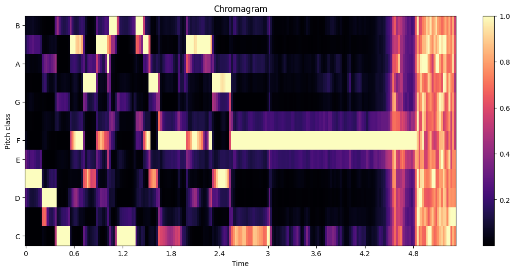
How to interpret the chromagram: Interpreting the Chromagram:

• The x-axis represents time.

• The y-axis represents the 12 pitch classes (C, C#, D, D#, E, F, F#, G, G#, A, A#, B).

• The color intensity represents the relative strength of each pitch class at each time point.

• Brighter colors indicate stronger presence of a pitch class.

Analyzing Chroma Features Over Time

Let’s look at how the intensity of each pitch class changes over time:

# Define pitch classes
pitch_classes = ['C', 'C#', 'D', 'D#', 'E', 'F', 'F#', 'G', 'G#', 'A', 'A#', 'B']

plt.figure(figsize=(14, 8))
for i in range(12):
    plt.subplot(4, 3, i+1)
    plt.plot(librosa.times_like(chroma), chroma[i])
    plt.title(pitch_classes[i])
    plt.xlabel('Time')
    plt.ylabel('Magnitude')
plt.tight_layout()
plt.show()

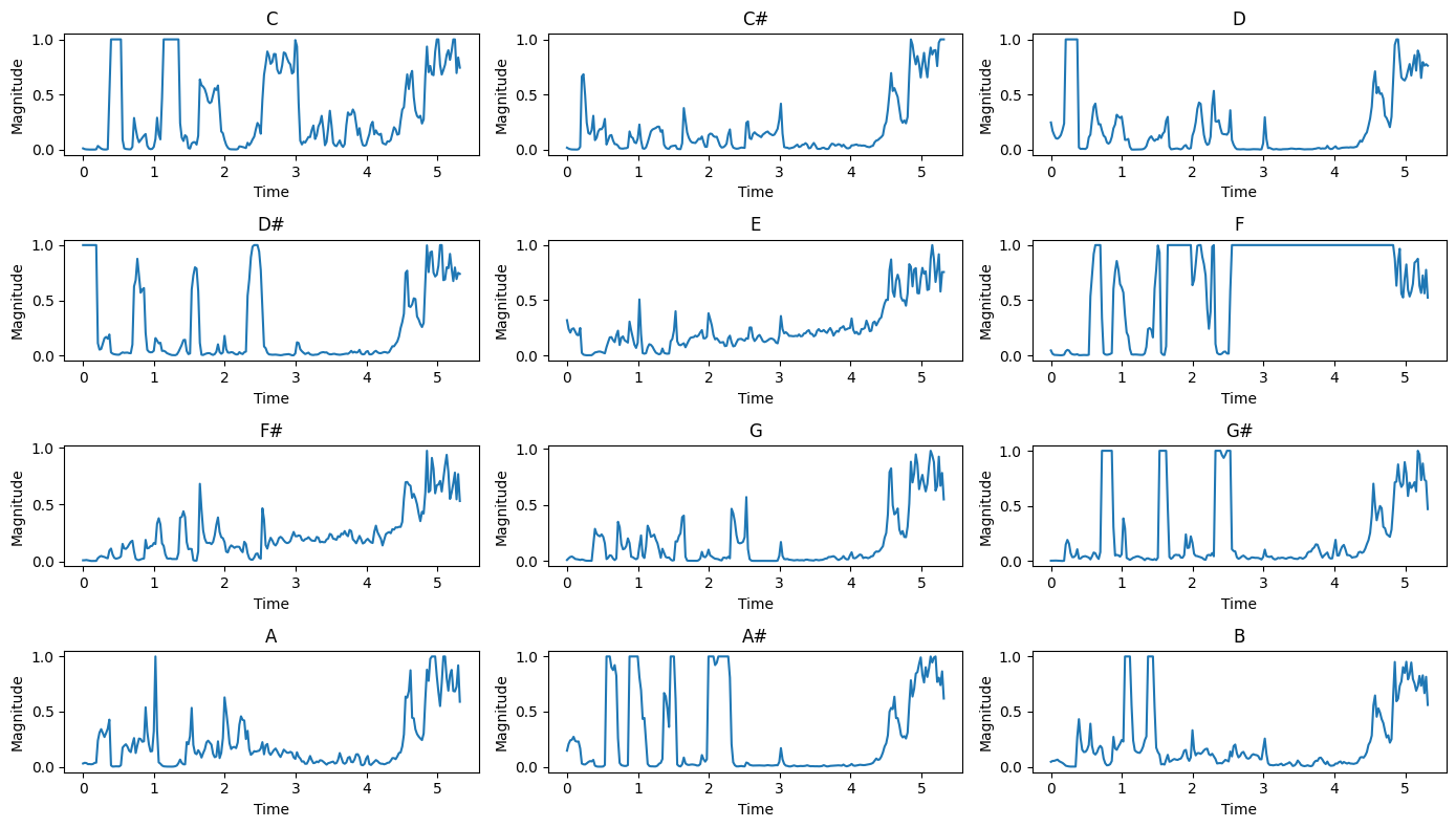
Observations:

• Peaks in these plots indicate strong presence of the corresponding pitch class.

• The patterns can reveal melodic and harmonic structures in the music.

• Sustained high values might indicate the key of the music or prominent chords.

Chroma Energy Normalized Statistics (CENS)

CENS features are a variant of chroma features that are more robust to variations in dynamics and timbre. They involve additional processing steps including local energy normalization and quantization.

# Compute CENS features
cens = librosa.feature.chroma_cens(y=y, sr=sr)

# Visualize CENS features
plt.figure(figsize=(14, 6))
librosa.display.specshow(cens, sr=sr, x_axis='time', y_axis='chroma')
plt.colorbar()
plt.title('Chroma Energy Normalized Statistics (CENS)')
plt.show()

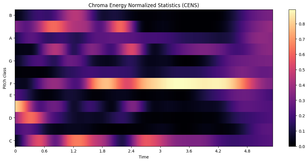
CENS features often provide a smoother representation of harmonic content, which can be beneficial for tasks like audio matching and cover song identification.

Chroma Features with Different Hop Lengths

The time resolution of chroma features can be adjusted by changing the hop length. Let’s compare chroma features computed with different hop lengths:

hop_lengths = [512, 2048, 4096]
plt.figure(figsize=(14, 12))

for i, hop_length in enumerate(hop_lengths):
    chroma = librosa.feature.chroma_stft(y=y, sr=sr, hop_length=hop_length)
    plt.subplot(3, 1, i+1)
    librosa.display.specshow(chroma, sr=sr, x_axis='time', y_axis='chroma', hop_length=hop_length)
    plt.colorbar()
    plt.title(f'Chromagram (hop_length = {hop_length})')

plt.tight_layout()
plt.show()

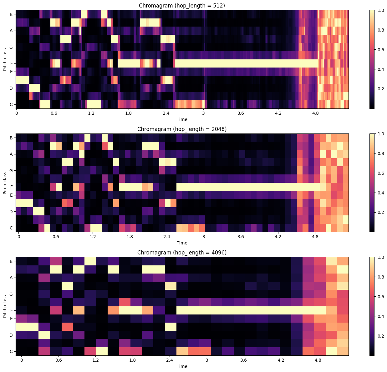
Observations:

• Smaller hop lengths provide higher time resolution but may be more sensitive to noise.

• Larger hop lengths provide a smoother representation but may miss rapid changes.

• The choice of hop length depends on the specific application and the nature of the audio signal.

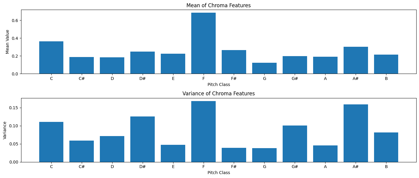
Chroma Feature Statistics

As with other features, it’s often useful to summarize chroma features using statistics. Let’s calculate the mean and variance of chroma features:

# Calculate statistics
chroma_means = np.mean(chroma, axis=1)
chroma_vars = np.var(chroma, axis=1)

# Display statistics
plt.figure(figsize=(14, 6))
plt.subplot(2, 1, 1)
plt.bar(pitch_classes, chroma_means)
plt.title('Mean of Chroma Features')
plt.xlabel('Pitch Class')
plt.ylabel('Mean Value')

plt.subplot(2, 1, 2)
plt.bar(pitch_classes, chroma_vars)
plt.title('Variance of Chroma Features')
plt.xlabel('Pitch Class')
plt.ylabel('Variance')

plt.tight_layout()
plt.show()

Applications of Chroma Features

Chroma features are widely used in various music information retrieval tasks, including:

• Chord Recognition: Identifying the chords played in a piece of music.

• Key Detection: Determining the musical key of a song.

• Music Structure Analysis: Identifying repeating sections, verse-chorus structures, etc.

• Cover Song Identification: Finding different versions of the same song.

• Music Similarity Measurement: Comparing harmonic content of different pieces.

• Melody Extraction: Isolating the main melodic line in polyphonic music.

Limitations of Chroma Features

While chroma features are powerful, they have some limitations:

• They discard octave information, which can be important for some applications.

• They may not capture non-harmonic aspects of music, such as rhythm or timbre.

• They can be affected by the presence of percussion or other non-pitched sounds.

• They assume equal temperament and may not accurately represent music from traditions with different tuning systems.

Section Summary

• Chroma features provide a powerful representation of the harmonic and tonal content of music.

• They capture information about pitch class distributions over time, which is crucial for many music analysis tasks.

• By being invariant to changes in octave, they offer a compact yet informative representation of musical content.

In this section, we’ve learned how to:

• Compute and visualize chroma features

• Analyze chroma features over time

• Compute Chroma Energy Normalized Statistics (CENS)

• Compare chroma features with different hop lengths

• Summarize chroma features using basic statistics

In combination with other audio features we’ve explored (like MFCCs for timbre and spectral features for overall frequency content), chroma features form part of a comprehensive toolkit for audio and music analysis.

The next steps in audio feature extraction might involve exploring more specialized features for specific tasks, or investigating how to combine different features effectively for various applications in music information retrieval and audio analysis.

In Practice: Combine Audio Features

In real-world audio processing applications, it’s often beneficial to combine multiple types of features to capture different aspects of the audio signal. This can lead to more robust and informative representations for machine learning models and other analysis tasks.

Here’s an example of combining the features we’ve explored in this tutorial:

def extract_features(y, sr):
    """
    Extract various audio features from an audio signal.
    
    Parameters:
    y (np.ndarray): Audio time series
    sr (int): Sampling rate
    
    Returns:
    dict: Dictionary of extracted features
    """
    features = {}
    
    # Time-domain features
    features['rms'] = librosa.feature.rms(y=y).mean()
    features['zcr'] = librosa.feature.zero_crossing_rate(y).mean()
    
    # Frequency-domain features
    spectral_centroid = librosa.feature.spectral_centroid(y=y, sr=sr)
    features['spectral_centroid'] = spectral_centroid.mean()
    spectral_rolloff = librosa.feature.spectral_rolloff(y=y, sr=sr)
    features['spectral_rolloff'] = spectral_rolloff.mean()
    
    # MFCCs
    mfccs = librosa.feature.mfcc(y=y, sr=sr, n_mfcc=13)
    for i, mfcc in enumerate(mfccs):
        features[f'mfcc_{i+1}'] = mfcc.mean()
    
    # Chroma features
    chroma = librosa.feature.chroma_stft(y=y, sr=sr)
    for i, pitch_class in enumerate(pitch_classes):
        features[f'chroma_{pitch_class}'] = chroma[i].mean()
    
    return features

# Extract features from the audio file
audio_features = extract_features(y, sr)
df = pd.DataFrame([audio_features]) # Convert to DataFrame.

df.T

	0
rms	0.052861
zcr	0.173491
spectral_centroid	2638.397724
spectral_rolloff	4410.983038
mfcc_1	-442.257904
mfcc_2	50.383911
mfcc_3	-70.578911
mfcc_4	-18.441648
mfcc_5	-16.287895
mfcc_6	-18.831705
mfcc_7	-21.320690
mfcc_8	-13.630634
mfcc_9	-20.642900
mfcc_10	-12.660918
mfcc_11	-9.462445
mfcc_12	-4.965589
mfcc_13	0.397866
chroma_C	0.349579
chroma_C#	0.180893
chroma_D	0.203917
chroma_D#	0.242832
chroma_E	0.247863
chroma_F	0.683089
chroma_F#	0.235193
chroma_G	0.159025
chroma_G#	0.233060
chroma_A	0.214012
chroma_A#	0.277623
chroma_B	0.206557

After extracting the features, we concatenate them along the feature axis to create a comprehensive feature matrix. This matrix can then be used as input to machine learning models, clustering algorithms, or other audio processing tasks.

Tips for Combining Audio Features

When working with combined feature sets, keep in mind the following:

• Curse of Dimensionality: As the number of features increases, the amount of data needed to make statistically sound inferences grows exponentially.

• Feature Selection: Not all features may be relevant for your specific task. Feature selection techniques can help identify the most informative features.

• Computational Complexity: Extracting and processing a large number of features can be computationally expensive, especially for real-time applications.

• Interpretability: While combined features can improve performance, they may make it harder to interpret the results in terms of audio characteristics.

Depending on the specific audio analysis task, you might combine features in different ways:

• Speech Recognition: Combine MFCCs with delta and delta-delta coefficients, energy features, and pitch-related features.

• Music Genre Classification: Combine MFCCs with chroma features, spectral features, and rhythm features.

• Speaker Identification: Use MFCCs along with formant frequencies, pitch features, and voice quality measures.

• Emotion Recognition: Combine MFCCs with prosodic features, pitch modulation features, and energy features.

• Audio Tokenization: Use MFCCs, Delta MFCCs, and Delta-Delta MFCCs as input features for tokenization models like Vector Quantization (VQ), VQ-VAE or Hidden Markov Models (HMM).

• Music Generation: Combine chroma features with rhythm features, MFCCs, and spectral features to capture different aspects of music content. You can then use these features as input to generative models like Variational Autoencoders (VAEs) or Generative Adversarial Networks (GANs).

Section Summary

Combining different types of audio features allows us to capture a more comprehensive representation of audio signals. This can lead to improved performance in various audio analysis tasks. However, it also introduces challenges in terms of feature selection, dimensionality reduction, and interpretation.

The process of feature extraction and combination is often iterative, involving experimentation with different feature sets and analysis techniques to find the best approach for a specific audio analysis task.

As you continue to work with audio features, consider exploring more advanced techniques such as:

• Deep learning-based feature extraction (e.g., using convolutional neural networks)

• Time-frequency representations like constant-Q transform or Mel-spectrograms

• Task-specific feature engineering based on domain knowledge

Remember that the choice of features and how they are combined should always be guided by the specific requirements of your audio analysis task and the characteristics of your dataset.

Next Steps

To further your understanding and application of audio feature extraction, consider exploring:

• Advanced Feature Extraction Techniques:

  • Constant-Q Transform

  • Gammatone Filterbanks

  • Tempogram for rhythm analysis

• Machine Learning with Audio Features:

  • Implement a classifier (e.g., SVM, Random Forest) using extracted features

  • Explore deep learning approaches like Convolutional Neural Networks for audio classification

• Real-time Audio Feature Extraction:

  • Implement feature extraction on streaming audio data

• Feature Selection and Engineering:

  • Investigate techniques for selecting the most relevant features for specific tasks

  • Create custom features based on domain knowledge

• Audio Data Augmentation:

  • Explore techniques for augmenting audio data to improve machine learning model performance

• Explore Other Audio Libraries:

  • Try other Python libraries like pyAudioAnalysis or essentia for audio feature extraction

• Large-scale Audio Analysis:

  • Apply these techniques to larger datasets

  • Explore distributed computing options for processing large audio collections

• Cross-domain Applications:

  • Investigate how audio features can be combined with other types of data (e.g., text, images) for multimodal analysis

Audio feature extraction is a rich and evolving field. Stay updated with the latest research and techniques. Experiment with new approaches as you tackle different audio analysis challenges.

References

• Extracting Features from Audio Samples for Machine Learning - A beginner-friendly guide to audio feature extraction.

• Audio Feature Extraction - Answers frequently asked questions about audio features.

• Music Information Retrieval: Fundamentals and Applications - A great book on music information retrieval techniques and applications.

• librosa: Audio and Music Signal Analysis in Python - The official documentation for librosa, the library used in this tutorial.