
Quantization#
TL;DR#
Quantization is a computational trick to make running AI models both possible and cheaper.
It’s specifically the process of taking a “very precise” number and making it less precise.
For example, 1.23123 versus 1.23.
Quantization can substantially reduce memory needs.
Practically speaking, it is basically required on consumer-grade hardware to run modern models.
Hugging Face’s Bits and Bytes library is quite common.
Quantization continues to be both an art and a science in the AI space.
Such as 1-bit LLMs.
A Simplified Summary#
Multiply 1.23112332 * 0.521341232.
Now do 70 billion more calculations, and you’ll have performed a single forward pass for a language model.
The next problem is doing those 70 billion calculations a couple thousand more times just to generate one response,
and we haven’t even gotten to training.
This huge number of calculations is why models require a relatively large amount of compute.
Aside from the calculations, the weights often need to fit into the memory of the available hardware,
and often this memory is not typical RAM but VRAM that is onboard an expensive GPU or TPU.
One of the most common tricks to make the compute faster,
and the memory requirements lower, is quantization.
Quantization essentially is this:
Instead of calculating 1.231 * 0.42134, we calculate 1.2 * 0.5.
The second calculation is much easier than the first,
one that requires fewer numbers to represent
and folks can do in their head.
From Hugging Face:
Quantization is a technique to reduce the computational and memory costs of running inference by representing the weights and activations with low-precision data types like 8-bit integer (int8) instead of the usual 32-bit floating point (float32).
API users can stop reading here#
If you access models through APIs, then that’s all you need to know about quantization. The LLM provider
If you’re deploying your own models, you’ll need to make a choice of which level to use. For instance, with Ollama, many quantization levels are available for each model. Here’s a subset of the Gemma 7B options.
As a first pass, you’ll need to pick a quantization level that fits the amount of memory you have available. However, past that, it becomes less obvious. With everything in GenAI, there is never a universal answer, as it depends on your situation. Understanding quantization in depth, though, will ensure you make an informed choice.
Quantization in Depth#
To really understand what’s going on with quantization, we need to dive into the fundamentals of computation, which are bits and bytes.
The core idea here is simple: In a world with constraints, to get something, we’re going to have to give something up.
In our case, we have a fixed amount of memory. Namely,
If we want to represent both negative and positive numbers, we lose the ability to represent some numbers.
There is a tradeoff between the “size of numbers” and precision.
In our LLM case, we need to make some decisions. Given we have so many numbers, do we favor range or precision for the limited amount of compute we have? To understand quantization, we’ll have to go back to the fundamentals, which is how computers represent numbers. We’ll start from the basics and build back up.
Basic Data Representation#
Most modern computers use binary, meaning they use either 0 or 1 to represent numbers.
If we have a 2-bit computer, we can count the numbers between 0 and 3 like this:
00 -> 0
01 -> 1
10 -> 2
11 -> 3
binary_list = ("0", "1", "10", "11")
To convert these to base 10,
which we normally use,
we can use Python’s built-in int function.
for binary_repr in binary_list:
    print(f"Binary: {binary_repr}, Base 10: {int(binary_repr, base=2)}")
Binary: 0, Base 10: 0
Binary: 1, Base 10: 1
Binary: 10, Base 10: 2
Binary: 11, Base 10: 3
Essentially, what’s happening is the position of the 0’s and 1’s is used to determine the exponent and the coefficient.
For a full explanation, see the Wikipedia page.
For our purposes, though, the only takeaway you need at this point is that with 2 bits, we can represent 4 possible numbers:
{0, 1, 2, 3}.
A binary joke
Computer nerds often say there are 10 types of people in the world: those who understand binary and those who don’t.
The good news: you’re now part of the former.
2 bits are quite limiting. Modern computers are much more powerful and can handle more bits. Commonly, 8 bits are grouped together into what’s called a byte, a unit of measurement you’ve heard of. Now we have enough “space” to represent integers all the way from 0 to 255.
Here’s some examples:
int("10000000", 2), 2**7 + 0*2**6 + 0*2**5 # etc.....
(128, 128)
int("11111111", 2), sum(2** i for i in range(8))
(255, 255)
bit_string_5 = "00000101"
int(bit_string_5, 2)
5
But What About Negative Numbers?#
So far, our numbers have been positive, but for LLMs and many other basic applications, we need negative numbers as well. To do this, we change the meaning of the first bit to be an indicator of sign.
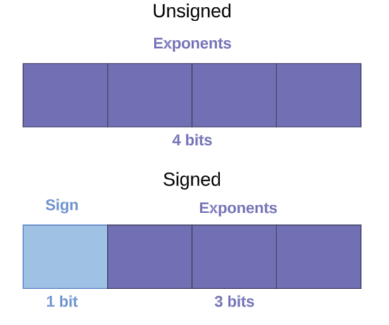
Fig. 41 Representing Unsigned and Signed Integers#
Here’s what it looks like in practice for 4 bits. The first bit now indicates whether the counting starts up from 0 or from -8. The tradeoff here is we shift the range of possible integers from 0 to 15 in unsigned, to -8 to 7 in signed representation.
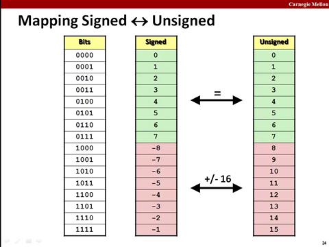
Fig. 42 4 bits binary table#
Here’s what this looks like for a byte string. We now need to provide some extra information, namely which bit is the signed bit, and whether the byte string is signed or not.
def byte_to_int(byte_str):
    """Converts a byte string to both its signed and unsigned integer representations."""
    bytes_obj = bytes([int(byte_str, base=2)])
    unsigned_int = int.from_bytes(bytes_obj, byteorder='big', signed=False)
    signed_int = int.from_bytes(bytes_obj, byteorder='big', signed=True)

    print(f"Signed int: {signed_int}, Unsigned int: {unsigned_int}")
    return
Let’s try this out in practice.
For our bit string of 5, we get the same number:
byte_to_int(bit_string_5)
Signed int: 5, Unsigned int: 5
If we flip the first bit to a 1, we now get two different numbers:
one counting 5 “up” from -128
and another counting 5 “up” from 128.
byte_to_int("10000101")
Signed int: -123, Unsigned int: 133
For a more in-depth explanation, this YouTube video explanation does a fantastic job with additional explanations.
Floating Point and Why Memory is Expensive#
Now, for GenAI, we need more than integers; we need floating point numbers. Let’s start with Float32. Per the IEEE 754, this is what each bit means.
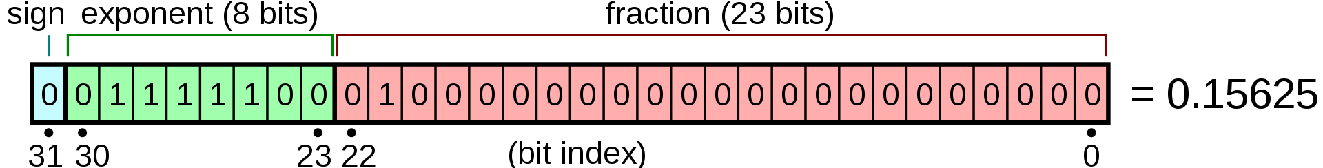
Fig. 43 How the bytes of a Float32 representation are laid out#
To represent floats, we now add a concept called the fraction. The exponent controls the scale, and the fraction controls the significant digits.
The fraction is also referred to as the significand or mantissa.
import struct
# https://docs.python.org/3/library/struct.html

# Example string of bits (32 bits for float32)
bits_string = '01000000101000000000000000000000'  # Example: 5.0 in float32 bits

# Convert binary string to bytes
int_value = int(bits_string, 2)

binary_data = int_value.to_bytes(4, byteorder='big')

# Unpack bytes into a float32
result = struct.unpack('>f', binary_data)

print(result)  # Output: 5.0
(5.0,)
You can try this out with any number using this handy floating point converter.
Quantization in Detail#
In the Floating Point 32 spec, 1 bit is for the sign, 8 bits are allocated to the exponent, and 23 bits to the mantissa. But do we need to use 32 bits? Can we change the number of bits allocated to the exponent and the mantissa?
The answer is no and yes. For machine learning, there are specialized formats such as bfloat16 that are specialized for ML/AI applications. By using 16 bits, the memory needs are already cut in half, and the larger allocation of bits to exponents allows for a wider range, though at the cost of precision.
We can get more memory savings by using 8-bit and 4-bit floats, and within those, similarly make trade-offs between the exponent and mantissa.
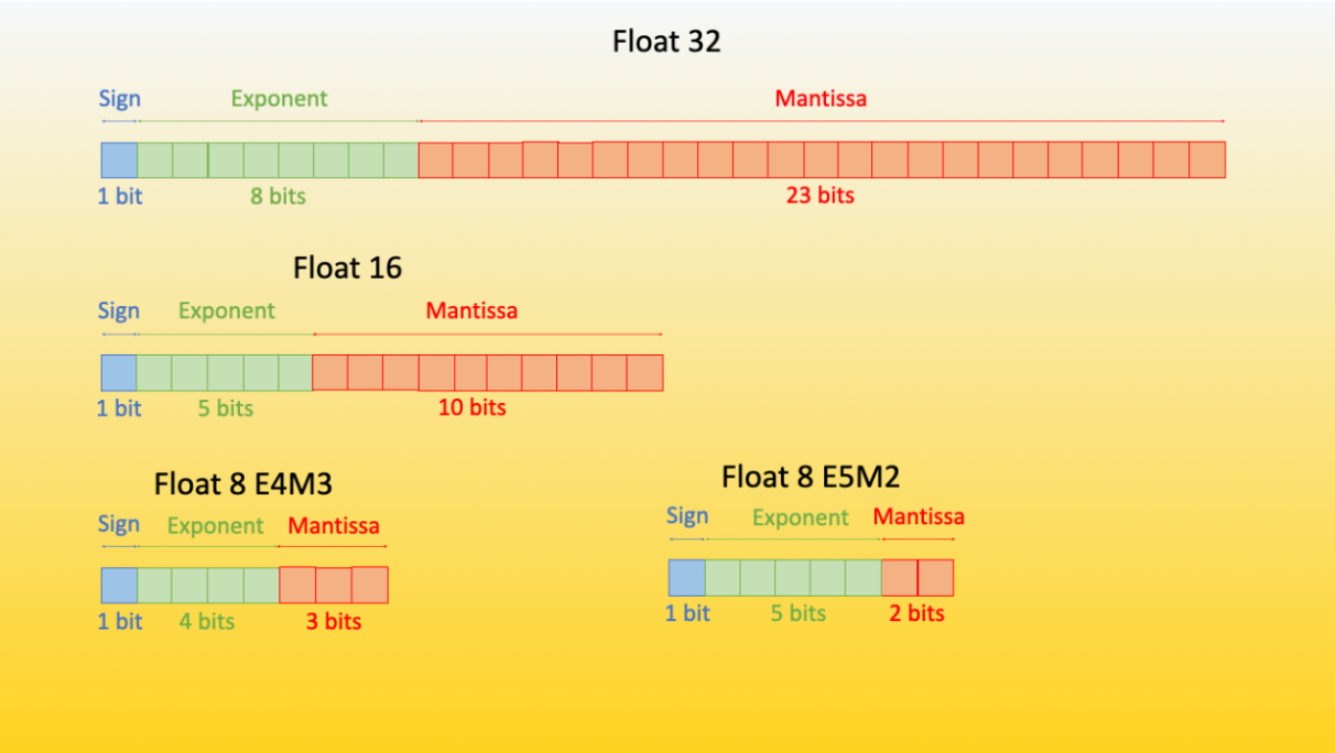
Fig. 44 The difference in bit size and allocation across 4 different formats in the Hugging Face Bits and Bytes library#
For those training LLMs, different data types can be used for the forward and backward pass. Hugging Face notes:
It has been empirically proven that the E4M3 is best suited for the forward pass, and the second version (E5M2) is best suited for the backward computation.
Practical Tips for Inference#
For Ollama users, the default Q4_0 works the best for me. The GGUF Q5_K_M, Q5_K_S, and Q4_K_M are the most recommended. However most useful quantization is the one that works. If only Q2 or Q3 works for your hardware, then you really have no choice. IF using LLMs in a high-stakes situation, such as a critical system or building an LLM startup, I suggest running a deeper evaluation against benchmarks or perplexity metrics such as the one shown here. Your use case likely merits the additional cost of larger hardware resources.
Active Field of Research#
How far quantization can go is an active field of research.
One research team took things to their logical extreme and created a ternary LLM where weights could only take on the values of {-1, 0, 1}.
They compared the performance of Bitnet against LLAMA Lookalike.
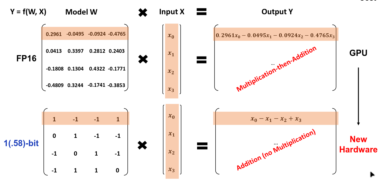
Fig. 45 Comparison of FP16 versus a trinary LLM from the 1.58 bit LLM paper#
1.58-bit model used substantially less memory while still having comparable performance. There are many different directions quantization can still take so we’ll see what papers come from future research efforts.
References#
BBC Guide on floating point format - A straightforward guide explaining the floating point format.
Wikipedia explaining significand - A longer explanation of the significand.
Wikibook full explanation of floating point format - A complete explanation of the fundamentals.
Little and Big Endian Formats - A succinct explainer of how this is represented.
Quantization Aware Training in Pytorch - A complete guide to quantization and QAT in a modern framework.
Bits and Bytes HF Transformers integration - Hugging Face Bits and Bytes that explains the motivation of integrating the library into Hugging Face transformers.
Bits and Bytes with QLORA - An explanation of quantized finetuning on low-powered hardware.
LLAMA.cpp issue showing quantization performance - Contains a great table that is directly useful for practitioners as many users use llama.cpp.
Practical advice on which quantization type to pick for Ollama users - Further details on setup for inference users.