Reinforcement Learning Basics

TLDR

• Ice Maze is a discrete fully observable environment with small action space

  • This makes it ideal starting point as it runs simply and is easy to inspect in a debugger

• This example contains implementations of all the key terminology from the intro, particularly some key distinctions.

  • For example reward vs return

• We choose a slightly more complex implementation of Q learning that includes advantage calculation.

  • While not necessary for a simple example this will prep us for PPO and GRPO in future chapters.

Show code cell content

Hide code cell content

import gymnasium as gym
import numpy as np
import os
import matplotlib.pyplot as plt
from cleanllm.rl.icemaze import plot

Basic RL Challenge: Ice Maze (Or Frozen Lake)

Ice maze is a classic RL setup, where our hero needs to get to a prize by navigating a maze. In this setup a small agent needs to learn how to navigate a maze with holes in the ice to find a rewards.

Fig. 24 Ice Maze agent navigating the maze Gymasium

The agent can move in all four directions, except when constrained by the board. Eventually the agent either falls in a hole and “loses”, or eventually gets to the prize and “wins”.

For us, the folks making the RL Algorithm we have three objectives.

1. Implement an algorithm where the agent learns to reach the prize

2. Implement an algorithm where the agent reaches the prizes in the least amount of steps

3. Ensure the learning is as computationally efficient as possible

Creating our Reinforcement Learning Setup

Below we’ll go through one algorithm, called Q Learning, and in this case with a Q table which is just a python dictionary and arrays.

While this simple setup will work with this small problems, with LLMs this simple implementation is not as possible. However our focus here though is not to learn the algorithm, but rather the specific terms and concepts as we’ll be using.

Ice Maze Choices

Policy

For the Ice Maze problem there are different choices and implementations that work. For the purpose of this tutorial we’ll choose Q-Learning which we implement here as an off-policy algorithm.

During training we’ll use an epsilon greedy behavior policy which sometimes deviates from the target policy which is the one we’ll use after training is complete to navigate the ice maze. In particular epsilon is the representation of explore vs exploit, another fundamental tradeoff in Reinforcement Learning. It represents how often we stick with our greedy policy of picking what is believed to be the best action, and how often we randomly do not and do something random.

def choose_action(q_table: np.ndarray, state: int, epsilon: float, env):
    """Chooses an action using an epsilon-greedy policy."""
    if np.random.uniform(0, 1) < epsilon:
        return env.action_space.sample() # Explore: pick a random action
    else:
        q_values = q_table[state]
        assert q_values.shape[0] == 4
        return np.argmax(q_values) # Exploit: pick the best known action

Value and Q-Value

This is the core of where our ice maze agent learns. We need to estimate the “goodness” of being in a state, or taking an action in a state. These are the Value and Q-Value respectively.

Quantities that are estimated:

• Return (Gt): The total discounted reward from time-step t. Gt = Rt+1 + 𝛾Rt+2 + …

• Value (V(s)): The expected return from a state s. V(s) = E[Gt|St=s].

• Q-Value (Q(s,a)): The expected return from taking an action a in a state s. Q(s,a) = E[Gt|St=s, At=a].

In our simple example, we update these values in a simple lookup table (a numpy array). The important concepts here are how “strongly” we update the values based on the reward given from the environment.

For this algorithm we have:

• Discount Factor (𝛾): How much to discount future rewards. A value close to 1 means we value future rewards highly.

• Learning Rate (α): How quickly we update our Q-table. A high learning rate means we give more weight to new information.

With Deep Q-Networks and LLMs, we’ll be updating a Neural Network’s weights using an optimizer instead of a table.

def update_q_table(
    q_table: np.ndarray, state: int, action: int, next_state: int, reward: float, alpha: float, gamma: float
):
    """
    Updates the action-value (Q-table) using the Q-learning rule.

    The agent's exploratory, 'off-policy' action is chosen in the
    `choose_action` function. This `update_q_table` function then provides
    the learning step.

    The learning rule is always greedy. It updates the value of the action
    taken (`action`) by looking at the best possible future value it can get
    from the `next_state` (i.e., `max(Q(next_state, a))`).

    This allows the agent to explore new actions while always learning and
    improving its estimate of the single, optimal policy.
    """
    old_expected_q_value = q_table[state, action] # Get the current value for the current state action pair
    # Assume that in the next state the model will pick the action with the max 
    next_max = np.max(q_table[next_state]) 

    # Temporal difference target is the reward of this state, plus a discounted assumption of the next max value
    td_target = reward + gamma * next_max

    # The error between the target and what we thought the target was
    td_error = td_target - old_expected_q_value

    # Update to an new adjusted value, but don't just snap to it. Apply another downweighting factor
    new_adjusted_q_value = old_expected_q_value + alpha * td_error
    q_table[state, action] = new_adjusted_q_value

Advantage

A challenge in reinforcement learning is high variance in the estimation of Q-values. Advantage is a concept that helps to mitigate this. The advantage of an action a in a state s is the difference between the Q-value for that action and the value of the state: A(s, a) = Q(s, a) - V(s).

The advantage tells us how much better it is to take a specific action a compared to the average action from that state. This can help in a few ways:

• Reduces variance: It can help to reduce the variance of policy gradient updates in more advanced algorithms.

• Better for learning: It can be more stable and efficient to learn the advantage instead of the Q-values directly.

While not strictly needed for Q-learning, it’s a fundamental concept in many modern RL algorithms.

def calculate_advantage(q_table):
    """Calculates the advantage table: A(s, a) = Q(s, a) - V(s)."""
    v_table = np.max(q_table, axis=1)
    return q_table - v_table.reshape(-1, 1)

Reinforcement Learning Loop

After all that here is the algorithm itself. The biggest choice here is number of episodes. This is how many times the model will try to traverse the maze.

# --- Main Script ---
env = gym.make("FrozenLake-v1", is_slippery=True)

# --- Hyperparameters ---
num_episodes = 10000
alpha = 0.1
gamma = 0.99
epsilon = 1.0
epsilon_decay_rate = 0.0001
min_epsilon = 0.01

# --- Frame Saving Setup ---
save_interval = 1000
output_dir = "output"
os.makedirs(output_dir, exist_ok=True)

# --- Identify Goal and Hole States ---
desc = env.unwrapped.desc.astype(str)
grid_size = desc.shape[0]
goal_coords = [(r, c) for r, row in enumerate(desc) for c, char in enumerate(row) if char == "G"]
hole_coords = [(r, c) for r, row in enumerate(desc) for c, char in enumerate(row) if char == "H"]

We initialize the q table here with zeros. This indicates that we don’t know any about the goodness of each state. We can also

q_table = np.zeros([env.observation_space.n, env.action_space.n])

From here we start the training loop, where the agent takes many actions, going through many states in thousands of episodes to finally learn the correct path.

from IPython.display import Image, display

# --- Training Loop ---
for episode in range(num_episodes):
    state, info = env.reset()
    terminated = False
    truncated = False
    trajectory = [state]
    
    while not terminated and not truncated:
        # Take an action and enter the next state and obtain a reward
        action = choose_action(q_table, state, epsilon, env)
        next_state, reward, terminated, truncated, info = env.step(action)

        # Update the q table based on the new information
        update_q_table(q_table, state, action, next_state, reward, alpha, gamma)

        # Update current state
        state = next_state
        trajectory.append(state)
    
        epsilon = max(min_epsilon, epsilon - epsilon_decay_rate)
        
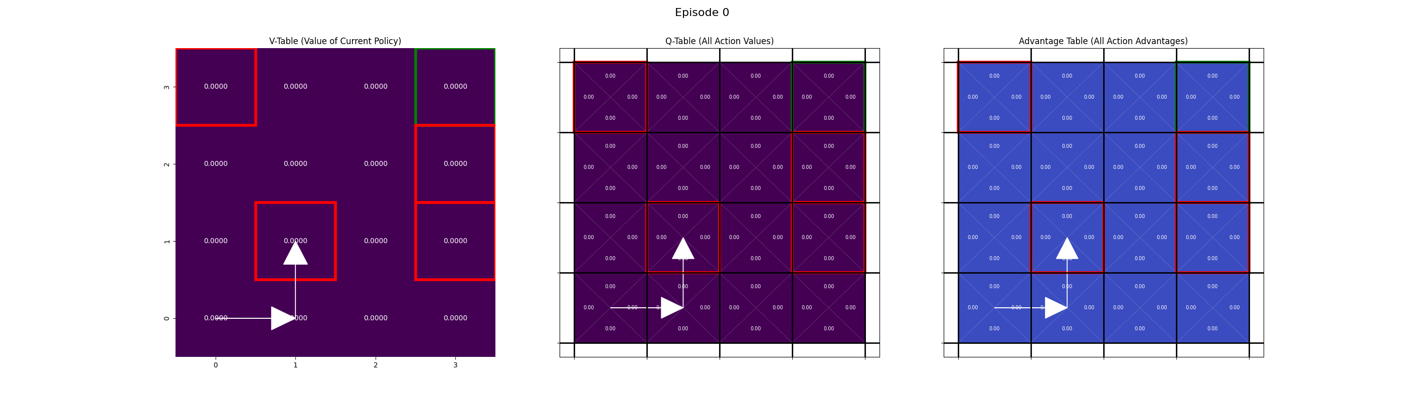
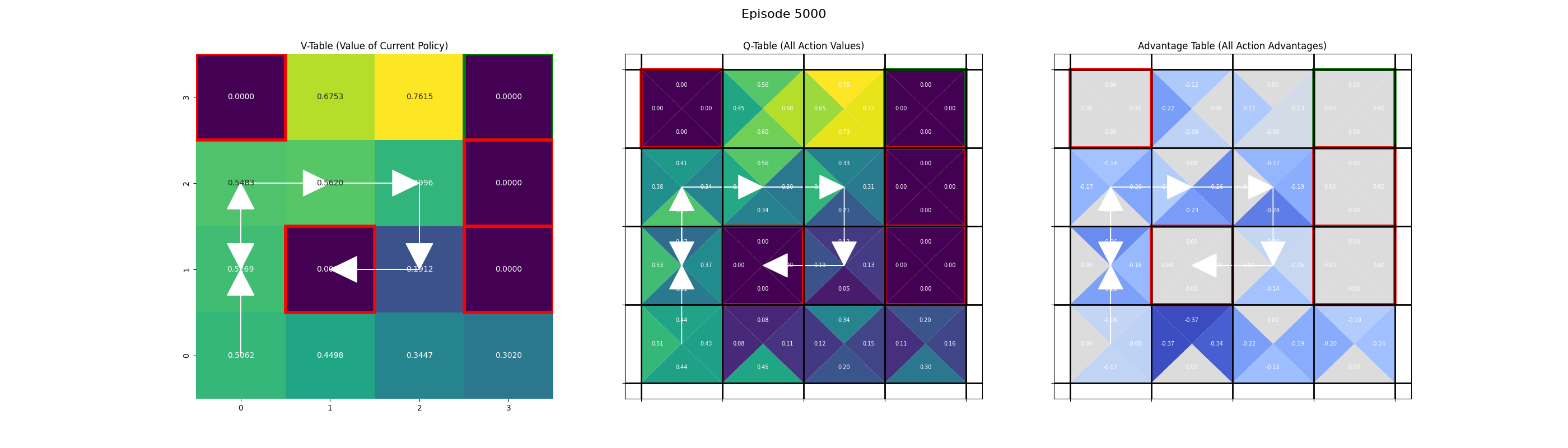
    # --- Save a frame at specified intervals ---    
    if episode % save_interval == 0 or episode == num_episodes - 1:
        print(f"Saving frame for episode {episode}...")
        advantage_table = calculate_advantage(q_table)
        value_table = np.max(q_table, axis=1)
        plot.save_frame(
            episode, value_table, q_table, advantage_table, trajectory, grid_size, goal_coords, hole_coords, output_dir
        )
        image_path = os.path.join(output_dir, f"episode_{episode}.png")
        display(Image(filename=image_path))

Saving frame for episode 0...

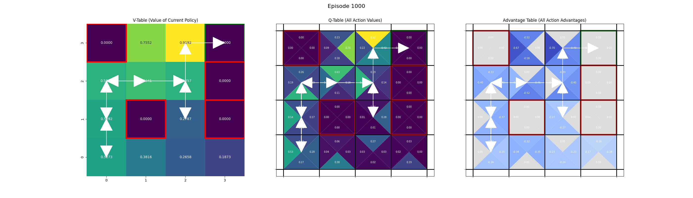
Saving frame for episode 1000...

Saving frame for episode 2000...

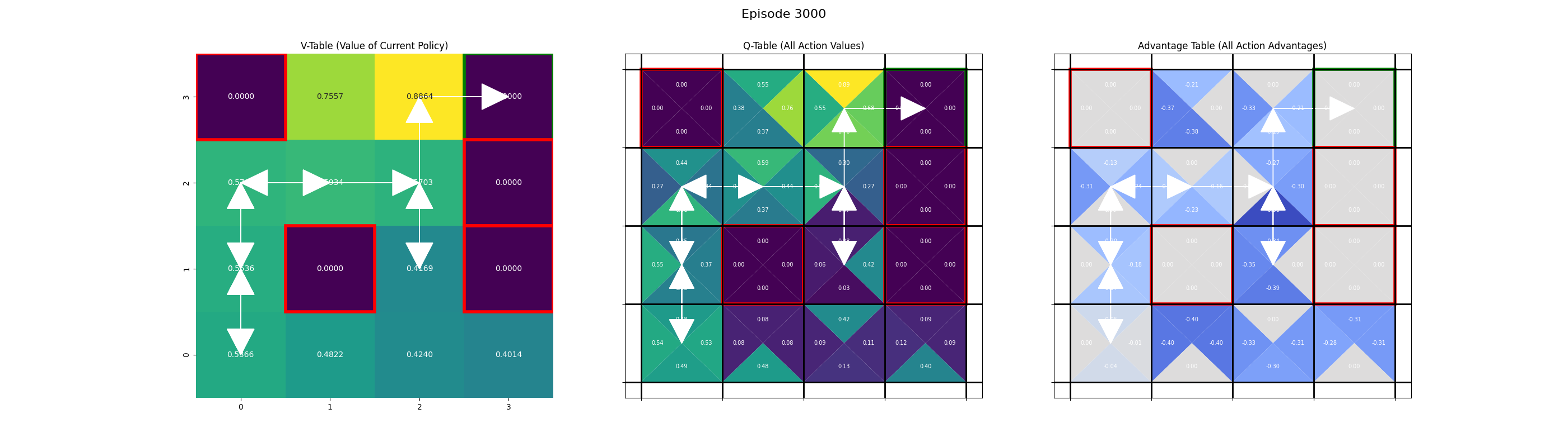
Saving frame for episode 3000...

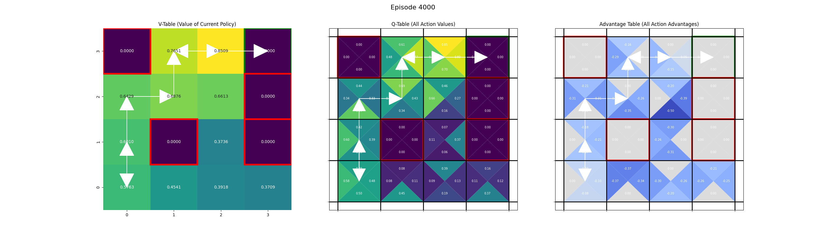
Saving frame for episode 4000...

Saving frame for episode 5000...

Saving frame for episode 6000...

Saving frame for episode 7000...

Saving frame for episode 8000...

Saving frame for episode 9000...

Saving frame for episode 9999...

Suggested Prompts

• What is the history of Reinforcement Learning?

• How has RL changed as models have become larger?

• What concepts in this notebook are used later in the LLM training chapters?

References

• Frozen Lake - Frozen Lake implementation from the Farama Foundation showing the setup of the challenge