
Neural Network Quickstart#
TLDR:
All statistical models are made of three parts:
A model that estimates things.
A way to measure how “bad” their estimates are.
A method to update the model parameters to make better estimates (hopefully).
Modern statistical models are coded in software
Enables scaling and iteration speeds never possible before.
Enables techniques for “guessing” new parameters through tools like autograd.
Neural networks are a type of statistical model
At their core, they are a lot of linear regression added together.
They’re put together in a way that can flexibly model all sorts of data.
This notebook contains all the code and libraries used for production scale LLMs
We use Jax to show you what the bare operations look like
We use Flax to show you the API that AI developers typically use
Neural Network Understanding From Linear Regression#
Neural network models are at the core of modern GenAI systems, including GenAI. If you zoomed into a single neuron in a neural network you’d see this.
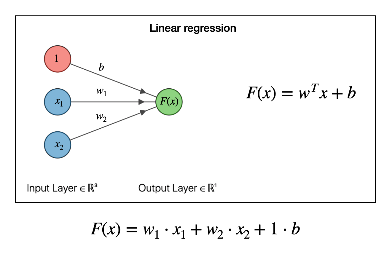
Fig. 1 The core of all AI models#
If it looks like a linear regression that’s exactly what it is. Now, with a model that’s \( y = mx + b \), or a single neuron, it by itself can’t predict much. But if you take a hundruds of thousands of of linear regressions and you structure them into this thing called a transformer, It’s mindboggling how this basic idea can be scaled and the end result is Artificial Intelligence.
There’s more than just the model#
However to really understand what’s going on you’ll need to know how to
Define a model
Measure its predictive performance
Update the parameters in a training loop.
For our linear model this is the steps look like.
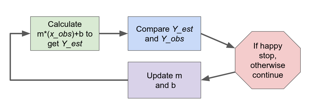
Fig. 2 How all AI models work#
If you’re comfortable with these concepts skip to training an LLM from scratch
But if you’re not we’re going to learn the basics by implementing a linear regression in Flax..
By starting a simple model though we can focus on the basics, before scaling up to LLM sized models.
From words to code.#
We’ll now implement a basic Linear Regression in Flax and the associated training loop in code.
Starting with our Linear Regression model we do the following:
Generate some toy data to work with
Create a linear regression model in Flax (a production Neural Network library that’s been used to train massive chat models)
Implement the parameter learning loop
Train the model
We’ll then extend our Linear Regression into a small neural network to show we can flexibly fit non linear data with a more complex model.
Run this Notebook Yourself!#
I encourage you to run this notebook to get hands-on practice and reinforce your learning. Use the colab button on the right to get going with one click. We’ll talk through fundamental concepts in words first. Then we’ll go through the same concepts end-to-end in code,
Simple Linear Regression#
import numpy as np
import jax
import jax.numpy as jnp
import matplotlib.pyplot as plt
import pandas as pd
from scipy import stats
Defining a model#
For our linear model.
\(m\) and \(b\) are the parameters we’re going to need to estimate.
\(x\) and \(y\) are what we observed and we’re going to use these to figure out what \(m\) and \(b\) should be.
In this example we’re going to expand this a bit and add one more coefficient. For those curious we do this for shape reasons.
These are the numbers that are the “ground truth” for our simulation. In this simple case we can verify that our learning process worked correctly by seeing it the model infers these parameters. Again In real life we never really know these parameters, but we can use parameter recvoery like this to debug our models.
Generate some observed y data#
We’re first going to generate some sample data to fit against. We do this because in real life we’ll never know the “true” answers, there might not even be one. By generating data ourselves we “know” the answers and we can verify that our model got it right.
m_0, m_1 = 1.1, 2.1
intercept = bias = 3.1
So now with \(m_0\), \(m_1\) and \(b\) set we can calculate what \(y\) will be if we pick any value of \(x_0\) and \(x_1\). Let’s pick some easy values first
# The shape needs to be (1,2). You'll see why below
coefficients = np.array([[m_0, m_1]])
x_0, x_1 = 0, 1
coefficients[0][0] * x_0 + coefficients[0][1] * x_1 + bias
5.2
x_0, x_1 = 1, 0
coefficients[0][0] * x_0 + coefficients[0][1] * x_1 + bias
4.2
Let’s pick some other values now to see what we get. Note how the values of the coefficients don’t change, it’s just x.
x_0, x_1 = 1.3, -2.5
coefficients[0][0] * x_0 + coefficients[0][1] * x_1 + bias
-0.7199999999999998
Generate Random X_0, X_1 points#
In real life we won’t always see numbers on a grid. To simulate this we generate x values at random places. We’ll use these x values to estimate our y values.
rng = np.random.default_rng(12345)
x_obs = rng.uniform(-10, 10, size=(200,2))
x_obs[:10]
array([[-5.45327955, -3.66483321],
       [ 5.94730915,  3.52509342],
       [-2.17780899, -3.34372144],
       [ 1.96617507, -6.26531629],
       [ 3.45512088,  8.83605731],
       [-5.03508571,  8.97762304],
       [ 3.34474906, -8.08204129],
       [-1.16320668,  7.72959839],
       [ 3.94907   , -3.47054272],
       [ 4.67856327, -5.59730089]])
Side Track: Fancy matrix multiplication#
So if we want to this with our first pair of x values and coefficients we could do it manually like this. But this is both ugly, error prone, and inefficient.
y_obs = coefficients[0][0] * x_obs[0][0] + coefficients[0][1] * x_obs[0][1] + bias
y_obs
-10.594757237912647
Matrix Multiplication#
So here’s a practical tip. If you’re going to work with Neural Nets you’re going to check shapes of things quite often. Let’s that here.
coefficients.shape, x_obs.shape
((1, 2), (200, 2))
With these two shapes we can do a matrix multiplication But if you remember from Linear Algebra class the dimensions have to match like this.
(1,2) @ (2, 200) = (1, 200)
Let’s go ahead and do that in code
# Typically done this way in NN literature so we get a column vector
y_obs = (x_obs @ coefficients.T) + bias
y_obs[:5]
array([[-10.59475724],
       [ 17.04473623],
       [ -6.31740492],
       [ -7.89437163],
       [ 25.45635331]])
Einsum is really nice#
We can also do the calculation above using einsum. This is an underrated features in most tensor libraries, so want to take this moment to show it to you here.
y_obs = np.einsum('ij,kj->ki', coefficients, x_obs) + bias
y_obs[:5]
array([[-10.59475724],
       [ 17.04473623],
       [ -6.31740492],
       [ -7.89437163],
       [ 25.45635331]])
Let’s add some noise to Y#
In real life we’ll never get exact measurements. Think of measuring something with a ruler or scale, there’s always a little bit of noise or error. To replicate this we add some random noise to our Y values.
noise_sd = .5
y_obs_noisy = y_obs + stats.norm(0, noise_sd).rvs(y_obs.shape)
What we’ve done up to this point#
So far we haven’t done any modeling yet. We’ve just generated some simulated data to work with.
We decided our data generated function is a two coefficient regression with a bias
\( y = m_0 * x_0 + m_1 * x_1 + b \)
Picked some arbitrary parameters
m_0, m_1 = 1.1, 2.1intercept = bias = 3.1
We picked some random x_0 and x_1 observations and calculated our y1_observations
In the real world we’d have observed this
weight = m1*height + m2+width
We generated some random x_0 and x_1 points
Used that to calculate Y
Added some random noise to Y
The real world is messy
Building a Model in Jax#
Let’s now code a model for our data. Reminder the goal here is to figure out the coefficients m_0, m_1, bias using our observed x_0, x_1, and y data.
Let’s do that using Jax and gradient descent. Gradient descent is important so let’s explain it here.
What is Jax#
Jax is a numerical library that enables
Very quick computation of mathematical operations
Automatic gradient calculation
For training Neural Networks both of these properties rae highly desirable, as we’ve mentioned, we want to quickly make estimates from our model, then figure out how to update the parameters so our estimates are better. Jax enables us to do both.
Estimating our parameters using gradient descent#
Start with some parameters that are probasbly nad
Make a prediction
Measure how bad that prediction is.
Figure out which way to adjust the parameters so the prediction is less bad
Change the parameters in direction
Go to Step 2 again
Repeas this until your your ability to make your guesses less bad stops.
This code block below contains
A model
A loss function
A gradient computation function
Model, Estimate, Loss Calculation and Training Loop#
Let’s now define all this in Jax and train our model.
import jax
import jax.numpy as jnp

# Generate sample data
X = jnp.array(x_obs)
Y = jnp.array(y_obs)

# Model definition
def model(params, X):
    weights = params["weights"]
    bias = params["bias"]
    return jnp.dot(X, weights) + bias

# Loss function
def mean_squared_error(params, X, Y):
    predictions = model(params, X)
    return jnp.mean((predictions - Y) ** 2)

# Initialize parameters
params = {'weights': jnp.zeros([2,1]), 'bias': 0.}

# Gradient descent optimizer
@jax.jit
def update(params, X, Y, learning_rate=0.001):
    loss_val, grads = jax.value_and_grad(mean_squared_error)(params, X, Y)
    print(X.shape)
    params = jax.tree_map(lambda p, g: p - learning_rate * g, params, grads)
    return loss_val, params

# Train the model
loss_vals = []
for _ in range(100):
    loss_val, params = update(params, X, Y)
    loss_vals.append(loss_val)

# Print final parameters
print("Learned weights:", params['weights'])
print("Learned bias:", params['bias'])
(200, 2)
Learned weights: [[1.0531881]
 [2.0895174]]
Learned bias: 0.5365327
fig, ax = plt.subplots()
ax.plot(range(100), loss_vals)
ax.set_ylabel("Loss Value")
ax.set_xlabel("Epoch or Step")
ax.set_title("Training Loss Curve");
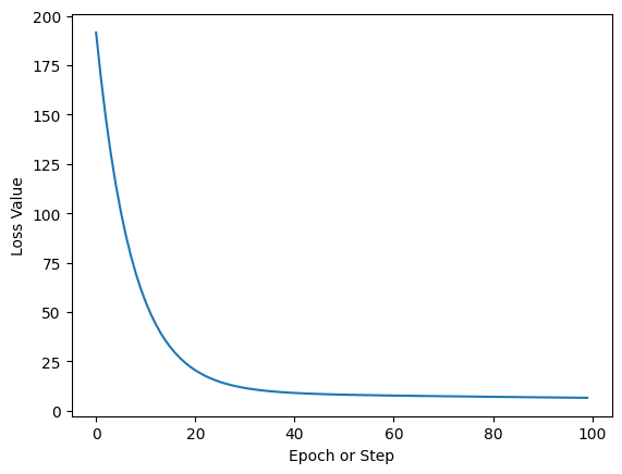
And that’s it. This curve shows how over a number of steps our computer is able to find parameters for our simple regression which produce better and better estimates. Once the curve flattens out this indicates there’s not much more to learn and we can stop the training loop.
Now let’s do this all again in Flax.
Building the same model in Flax#
With simple things like linear regression writing code by hand is fine. But when writing larger neural networks doing this by hand becomes tedious and error prone.
Flax is a neural network library that has been used to some of the biggest models in the world. Now using Flax for a simple linear regression is a bit of an overkill, like driving a semi truck to pick up a carton of milk at the grocery store. But it’ll do the job as you’ll see below.
import flax.linen as nn
class LinearRegression(nn.Module):
    # Define the neural network architecture
    def setup(self):
        """Single output, I dont need to specify shape"""
        self.dense = nn.Dense(features=1)

    # Define the forward pass
    def __call__(self, x):
        y_pred = self.dense(x)
        return y_pred
model = LinearRegression()
key = jax.random.PRNGKey(0)
An NVIDIA GPU may be present on this machine, but a CUDA-enabled jaxlib is not installed. Falling back to cpu.
Initialize Random Parameters#
params = model.init(key, x_obs)
params
{'params': {'dense': {'kernel': Array([[ 0.23232014],
          [-1.5953745 ]], dtype=float32),
   'bias': Array([0.], dtype=float32)}}}
Print Model Architecture#
print(model.tabulate(key, x_obs,
      console_kwargs={'force_terminal': False, 'force_jupyter': True}))
                              LinearRegression Summary
┏━━━━━━━┳━━━━━━━━━━━━━━━━━━┳━━━━━━━━━━━━━━━━┳━━━━━━━━━━━━━━━━┳━━━━━━━━━━━━━━━━━━━━━━┓
┃ path  ┃ module           ┃ inputs         ┃ outputs        ┃ params               ┃
┡━━━━━━━╇━━━━━━━━━━━━━━━━━━╇━━━━━━━━━━━━━━━━╇━━━━━━━━━━━━━━━━╇━━━━━━━━━━━━━━━━━━━━━━┩
│       │ LinearRegression │ float32[200,2] │ float32[200,1] │                      │
├───────┼──────────────────┼────────────────┼────────────────┼──────────────────────┤
│ dense │ Dense            │ float32[200,2] │ float32[200,1] │ bias: float32[1]     │
│       │                  │                │                │ kernel: float32[2,1] │
│       │                  │                │                │                      │
│       │                  │                │                │ 3 (12 B)             │
├───────┼──────────────────┼────────────────┼────────────────┼──────────────────────┤
│       │                  │                │          Total │ 3 (12 B)             │
└───────┴──────────────────┴────────────────┴────────────────┴──────────────────────┘

                             Total Parameters: 3 (12 B)
With a model defined we can pick values of x and see what we get for y.
x1, x2 = 1, 0
model.apply(params, [1,0])
Array([0.23232014], dtype=float32)
L2 Loss by Hand#
We’re going to use L2 loss, also know as mean squared error. This is a common error metric, but definitely not the only one.
m = params["params"]["dense"]["kernel"]
m
Array([[ 0.23232014],
       [-1.5953745 ]], dtype=float32)
bias = params["params"]["dense"]["bias"]
m = params["params"]["dense"]["kernel"]
y_0_pred = m[0] * x_obs[0][0] + m[1] * x_obs[0][1] + bias
y_0_pred
Array([4.5798745], dtype=float32)
y_obs[0]
array([-10.59475724])
(y_0_pred - y_obs[0])**2 / 2
Array([115.13471], dtype=float32)
Use Optax instead#
Common loss functions like L2 are already defined in libraries like optax, so rather than having to handcode them we can just import and run them.
import optax
y_pred = model.apply(params, x_obs[0])
y_pred
Array([4.5798745], dtype=float32)
y_pred = model.apply(params, x_obs[0])

optax.l2_loss(y_pred[0], y_obs[0][0])
Array(115.13471, dtype=float32)
Training Loop#
from flax.training import train_state # Useful dataclass to keep train state
# Note so jax needs to differentiate this
@jax.jit
def flax_l2_loss(params, x, y_true):
    y_pred = model.apply(params, x)
    total_loss = optax.l2_loss(y_pred, y_true).sum()

    return total_loss

flax_l2_loss(params, x_obs[0], y_obs[0])
Array(115.13471, dtype=float32)
optimizer = optax.adam(learning_rate=0.001)
state = train_state.TrainState.create(apply_fn=model, params=params, tx=optimizer)
type(state)
flax.training.train_state.TrainState
state
TrainState(step=0, apply_fn=LinearRegression(), params={'params': {'dense': {'kernel': Array([[ 0.23232014],
       [-1.5953745 ]], dtype=float32), 'bias': Array([0.], dtype=float32)}}}, tx=GradientTransformationExtraArgs(init=<function chain.<locals>.init_fn at 0x7ff70c54a340>, update=<function chain.<locals>.update_fn at 0x7ff70c54a200>), opt_state=(ScaleByAdamState(count=Array(0, dtype=int32), mu={'params': {'dense': {'bias': Array([0.], dtype=float32), 'kernel': Array([[0.],
       [0.]], dtype=float32)}}}, nu={'params': {'dense': {'bias': Array([0.], dtype=float32), 'kernel': Array([[0.],
       [0.]], dtype=float32)}}}), EmptyState()))
epochs = 10000
_loss = []

for epoch in range(epochs):
    # Calculate the gradient
    loss, grads = jax.value_and_grad(flax_l2_loss)(state.params, x_obs, y_obs_noisy)
    _loss.append(loss)
    # Update the model parameters
    state = state.apply_gradients(grads=grads)
Training Loss#
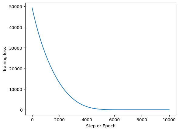
fig, ax = plt.subplots()
ax.plot(np.arange(epochs), _loss)
ax.set_xlabel("Step or Epoch")
ax.set_ylabel("Trainng loss");
Final Parameters#
With all that we now have our final parameters. Reference these against the coefficients we set above.
state.params
{'params': {'dense': {'bias': Array([3.1378474], dtype=float32),
   'kernel': Array([[1.1043512],
          [2.0921109]], dtype=float32)}}}
What if our data is non linear?#
So in our previous case we knew the relationship between x and y was linear because we generated it. In reality though most relationships are quite non linear, for example the relation between the pixels of an image, and the image being a cat. Or the relation between words in a sentence.
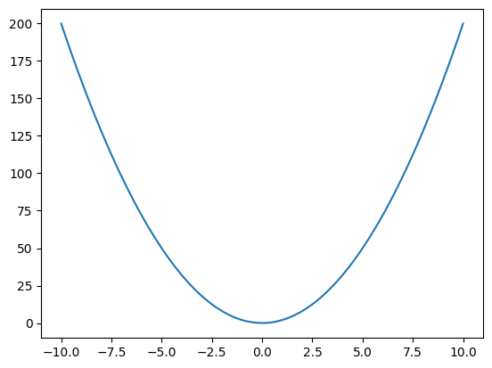
Here we’ll once again simulate data but this time with a non linear relationship between x and y.
x_non_linear = np.linspace(-10, 10, 100)
m = 2
y_non_linear = m*x_non_linear**2
fig, ax = plt.subplots()
ax.plot(x_non_linear,y_non_linear);
Initialize Params for our model#
params = model.init(key, x_non_linear)
params["params"]["dense"]["kernel"].shape
(100, 1)
We need to reshape X#
x_non_linear[..., None][:5]
array([[-10.        ],
       [ -9.7979798 ],
       [ -9.5959596 ],
       [ -9.39393939],
       [ -9.19191919]])
params = model.init(key, x_non_linear[..., None])
params
{'params': {'dense': {'kernel': Array([[-0.92962414]], dtype=float32),
   'bias': Array([0.], dtype=float32)}}}
state = train_state.TrainState.create(apply_fn=model, params=params, tx=optimizer)
type(state)
flax.training.train_state.TrainState
epochs = 10000
_loss = []

for epoch in range(epochs):
    # Calculate the gradient, shapes are really annoying
    loss, grads = jax.value_and_grad(flax_l2_loss)(state.params, x_non_linear[..., None], y_non_linear[..., None])
    _loss.append(loss)

    # Update the model parameters
    state = state.apply_gradients(grads=grads)
state.params
{'params': {'dense': {'bias': Array([9.870098], dtype=float32),
   'kernel': Array([[-7.460363e-08]], dtype=float32)}}}
y_pred = model.apply(state.params, x_non_linear[..., None])
y_pred[:5]
Array([[9.870099],
       [9.870099],
       [9.870099],
       [9.870099],
       [9.870099]], dtype=float32)
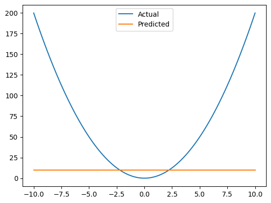
This is a terrible fit#
If we plot our original data, and what out model is able to estiate, we see that’s it’s not close at all. Our model can only really fit a line, but it’s too simplisitic to fit a parabola.
fig, ax = plt.subplots()
ax.plot(x_non_linear, y_non_linear, label="Actual")
ax.plot(x_non_linear, y_pred, label="Predicted")
ax.legend();
Expanding our model#
Let’s expand our neural network so it can more flexibly fit data.
We do this by adding a second layer.
We also incrase the number of parameters using the features keyword.
We also include the a relu layer.
This is known as an activation function in a Neural Network.
It’s what let’s individual neurons turn themselves “on” or “off”
class NonLinearRegression(nn.Module):
    # Define the neural network architecture
    def setup(self):
        """Single output, I dont need to specify shape"""
        self.hidden_layer_1 = nn.Dense(features=4)
        self.hidden_layer_2 = nn.Dense(features=4)
        self.dense_out = nn.Dense(features=1)

    # Define the forward pass
    def __call__(self, x):
        hidden_x_1 = self.hidden_layer_1(x)
        hidden_x_2 = self.hidden_layer_2(hidden_x_1)
        x = nn.relu(hidden_x_2)
        y_pred = self.dense_out(x)
        return y_pred
model = NonLinearRegression()
params = model.init(key, x_non_linear[..., None])
params
{'params': {'hidden_layer_1': {'kernel': Array([[-1.3402965 ,  0.60816777, -0.06039568, -0.73402834]], dtype=float32),
   'bias': Array([0., 0., 0., 0.], dtype=float32)},
  'hidden_layer_2': {'kernel': Array([[ 0.4993827 , -0.15674856,  0.19190995, -0.7276566 ],
          [-0.16007023,  0.4871689 , -0.32242206,  0.20559888],
          [ 1.0811065 , -0.07486992, -0.2228159 ,  0.18825608],
          [-1.068188  , -0.01827471, -0.34845108, -0.7157423 ]],      dtype=float32),
   'bias': Array([0., 0., 0., 0.], dtype=float32)},
  'dense_out': {'kernel': Array([[-0.4820224 ],
          [-0.11561313],
          [-1.0410513 ],
          [-0.37862116]], dtype=float32),
   'bias': Array([0.], dtype=float32)}}}
state = train_state.TrainState.create(apply_fn=model, params=params, tx=optimizer)
epochs = 3000
_loss = []

for epoch in range(epochs):
    # Calculate the gradient. Also shapes are really annoying
    loss, grads = jax.value_and_grad(flax_l2_loss)(state.params, x_non_linear[..., None], y_non_linear[..., None])
    _loss.append(loss)
    # Update the model parameters
    state = state.apply_gradients(grads=grads)
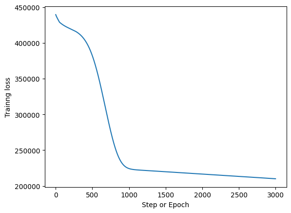
fig, ax = plt.subplots()
ax.plot(np.arange(epochs), _loss)
ax.set_xlabel("Step or Epoch")
ax.set_ylabel("Trainng loss");
Calculate Predictions#
y_pred_non_linear = model.apply(state.params, x_non_linear[..., None])
Plot Predictions#
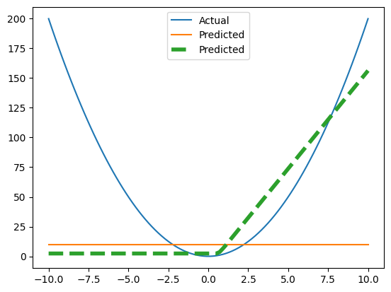
So here’s our fit. It’s better but it’s not great.
fig, ax = plt.subplots()
ax.plot(x_non_linear, y_non_linear, label="Actual");
ax.plot(x_non_linear, y_pred, label="Simple Model Predictions", ls='--');
ax.plot(x_non_linear, y_pred_non_linear, label="More Complex Predictions", ls='--', lw=2)
plt.legend();
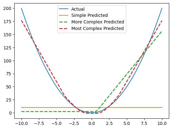
Non Linear (but more complex)#
Let’s now fit another model but we’ll increase the complexity by adding many more features, 128 in this case. Notice how the model is now able to fit the parabola “better”. It’s not perfect but this is the idea. Get a really big model with a lot of parameters and it theoretically find the structure in anything, even the words on the internet in every language, including code.
class NonLinearRegression_2(nn.Module):

    # Define the neural network architecture
    @nn.compact
    def __call__(self, x):
        x = nn.Dense(128)(x)              # create inline Flax Module submodules
        x = nn.relu(x)
        x = nn.Dense(features=1)(x)       # shape inference
        return x
model = NonLinearRegression_2()
params = model.init(key, x_non_linear[..., None])
state = train_state.TrainState.create(apply_fn=model, params=params, tx=optimizer)
epochs = 3000
_loss = []

for epoch in range(epochs):
    # Calculate the gradient. Also shapes are really annoying
    loss, grads = jax.value_and_grad(flax_l2_loss)(state.params, x_non_linear[..., None], y_non_linear[..., None])
    _loss.append(loss)
    # Update the model parameters
    state = state.apply_gradients(grads=grads)
y_pred_non_linear_2 = model.apply(state.params, x_non_linear[..., None])
fig, ax = plt.subplots()
ax.plot(x_non_linear, y_non_linear, label="Actual");
ax.plot(x_non_linear, y_pred, label="Simple Model Predictions", ls='--');
ax.plot(x_non_linear, y_pred_non_linear, label="More Complex Predictions", ls='--', lw=2)
ax.plot(x_non_linear, y_pred_non_linear_2, label="Most Complex Predicted", ls='--', lw=2)

plt.legend();
That’s all there is to create Neural Nets and LLMs. With that you’re ready for the next notebook where we recreate a Shakespeare LLM from scratch using the same tools here.
References#
NN are just linear regressions - An extended explanation of how these two are related
Why we want multi layer Neural Networks - A short video showing how multi layer neural networks do a better job fitting odd data, though sometimes too good of a job
Flax Docs - Aside from API documentation there’s also many examples of various other types of neural networks.