TL;DR
Diffusion Models are neural networks that generate images by gradually denoising random patterns.
The process involves two main steps:
Forward: Adding noise to an image
Reverse: Removing noise to recover the original image
Diffusion models have gained popularity due to their high-quality outputs and stable training.
Power popular AI art tools like
Stable Diffusion
DALL-E
Midjourney
Google’s Imagen
Key advantages:
Higher quality outputs than GANs/VAEs
More stable training
Better control over generation
Real-world uses:
Image creation
Video editing
Speech synthesis
Introduction
Imagine taking a photograph and slowly adding random dots of noise until the image becomes completely unrecognizable – like static on an old TV. Now imagine having an AI that can reverse this process, starting with pure noise and gradually transforming it into a clear, detailed image. This is essentially how diffusion models work, and they’re revolutionizing the world of AI-generated content.
What are Diffusion Models?
Diffusion models are a class of deep learning models that learn to generate data by gradually denoising a random signal. Unlike their predecessors (GANs and VAEs), diffusion models:
Work by learning to reverse a gradual noising process
Produce higher quality and more diverse outputs
Are more stable during training
Have strong mathematical foundations
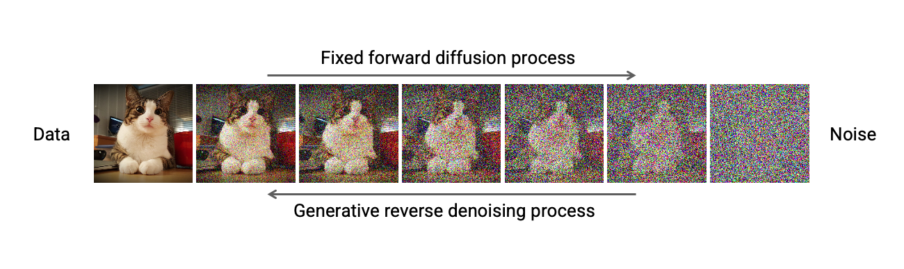
Figure 1:The diffusion process: From a clear image to noise (forward) and from noise to a clear image (reverse). Source
Why They Matter Now
Diffusion models have exploded in popularity since 2020 due to several breakthrough developments:
DDPM Breakthrough
Core Architectures
State-of-the-art Results: They’re behind many leading image generation systems:
Architecture Innovations
Key Advantages:
Higher image quality than previous methods
Better control over the generation process
More stable training
Stronger theoretical foundations
Real-World Applications
Diffusion models have found widespread applications across various domains in AI. Here’s an overview of some key applications:
| Application | Description |
|---|---|
| Text-to-Image Synthesis | Diffusion models like SDXL have achieved state-of-the-art results in generating high-resolution images from text prompts, offering improved visual fidelity and diversity. [1] |
| Video Editing | Dreamix, a diffusion-based method, enables text-based motion and appearance editing of general videos, combining low-resolution spatio-temporal information with newly synthesized high-resolution details. [2] |
| Speech Synthesis | NaturalSpeech 2 leverages diffusion models for zero-shot speech and singing synthesis, outperforming previous text-to-speech systems in prosody, timbre similarity, and voice quality. [3] |
| Image Enhancement | The Pyramid Diffusion model (PyDiff) addresses low-light image enhancement, using a novel pyramid diffusion method to progressively increase resolution during the reverse process. [4] |
| Adversarial Purification | DiffPure employs diffusion models to remove adversarial perturbations from images, demonstrating superior performance compared to traditional adversarial training methods. [5] |
| Controllable Generation | Loss-Guided Diffusion (LGD) enables plug-and-play controllable generation by guiding diffusion models with differentiable loss functions, applicable to tasks like image super-resolution and conditional image generation. [6] |
The Basic Concept
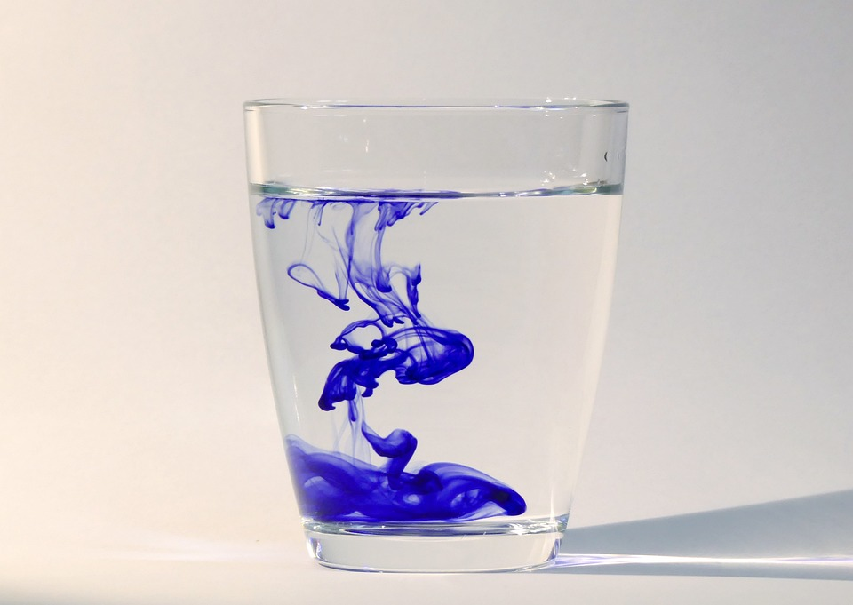
Imagine a drop of ink in water. Naturally, the ink gradually diffuses until the water becomes uniformly cloudy. Now imagine being able to reverse this process - starting with cloudy water and making the ink reform into its original shape. This is conceptually similar to how diffusion models work with images.
| Process | Description | Mathematical Form | Explanation |
|---|---|---|---|
| Forward | Adding noise | - q: Forward process - x_t: Image at current timestep - x_{t-1}: Image at previous timestep - | means “conditional on” or “given” | |
| Reverse | Removing noise | - p_θ: Reverse process (θ is neural network parameters) - x_{t-1}: Less noisy image we want to predict - x_t: Current noisy image |
The Forward Diffusion Process
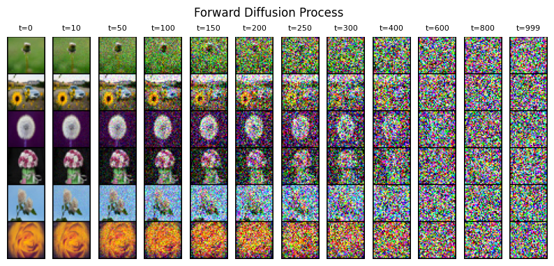
Figure 3:The forward diffusion process: Gradually adding noise to an image until it becomes pure random noise. Source
The forward process happens in small steps (typically 1000):
Step 0: Start with a clear image
Step 1-999: Add small amounts of Gaussian noise
Step 1000: End with pure random noise
Key characteristics:
Completely destroys image information
Process is fixed (not learned)
Each step adds a predictable amount of noise
Understanding the Mathematics
The full equation for a forward diffusion step is:
Where:
is the image at the current timestep
is the image at the previous timestep
(alpha) controls how much noise is added at each step
multiplies the image content
multiplies the noise
is random Gaussian noise
decreases over time to gradually add more noise
def forward_diffusion_step(x_previous, timestep):
    """
    x_previous: Image at previous timestep (x_{t-1})
    timestep: Current position in diffusion process (t)
    """
    noise = torch.randn_like(x_previous)  # Random Gaussian noise (ε)
    alpha_t = get_alpha(timestep)         # Get noise schedule value (α_t)

    # Apply the forward diffusion formula
    x_current = sqrt(alpha_t) * x_previous + sqrt(1 - alpha_t) * noise
    return x_current
The Reverse Diffusion Process
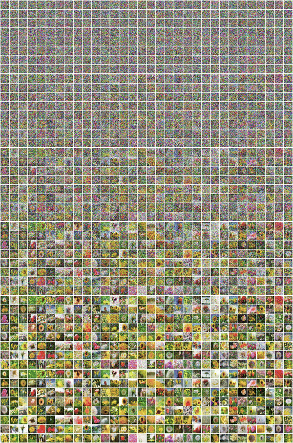
Figure 4:The reverse diffusion process: Gradually removing noise to recover the original image. Source
This is where the magic happens. The model learns to reverse the forward process:
Start: Pure random noise
Middle stages: Increasingly recognizable forms
End: Clear, detailed image
The reverse process is more complex than the forward process because it needs to predict and remove noise. The key equation for reverse diffusion is:
Where:
is the reverse process with learned parameters θ
is the less noisy image we want to predict
is the current noisy image
represents a normal (Gaussian) distribution
is the predicted mean (denoised image)
is the variance at timestep t
is the identity matrix
The neural network predicts the noise , which is then used to compute the denoised image:
Where:
is the noise schedule parameter at timestep t
is the cumulative product of alphas up to timestep t
is the predicted noise from the neural network
def reverse_diffusion_step(x_current, timestep, model):
    """
    x_current: Current noisy image (x_t)
    timestep: Current position in diffusion process (t)
    model: Neural network that predicts noise
    """
    # Get schedule parameters
    alpha_t = get_alpha(timestep)
    alpha_bar = get_cumulative_alpha(timestep)

    # Predict noise using the model
    predicted_noise = model(x_current, timestep)

    # Calculate the denoised image using the formula
    x_previous = (1 / sqrt(alpha_t)) * (
        x_current -
        ((1 - alpha_t) / sqrt(1 - alpha_bar)) * predicted_noise
    )

    return x_previous
Key characteristics of the reverse process:
Uses a U-Net architecture to predict noise
Each step removes a small amount of noise
The process is guided by the learned parameters θ
Can be conditioned on additional information (like text prompts)
The complete reverse process involves:
Starting with random noise
Iteratively applying the reverse step T times
Ending with the predicted clean image
This iterative process gradually transforms random noise into a coherent image, guided by the learned understanding of how to remove noise at each step.
Why This Approach Works
The diffusion approach has several advantages:
Gradual Changes
Small steps make the problem easier to learn
Each step only needs to remove a tiny bit of noise
Mathematical Tractability
The process can be described precisely
Training objectives are well-defined
Controlled Generation
The step-by-step nature allows for better control
Can intervene at any point in the process
Important Terminology
| Term | Definition |
|---|---|
| Timestep | Position in the diffusion process (t=0 to T) |
| Noise Schedule | Plan for how much noise to add at each step |
| Sampling | Process of generating new images |
| Denoising | Removing noise to recover the image |
Diffusion Model Types
Diffusion models have evolved into several distinct types, each with unique characteristics and applications. Here’s an overview of the main types of diffusion models:
| Type | Description |
|---|---|
| Denoising Diffusion Probabilistic Models (DDPMs) | The foundational diffusion model type that learns to reverse a gradual noising process through a series of denoising steps[7] |
| Latent Diffusion Models (LDMs) | Operate in a compressed latent space, reducing computational costs while maintaining high-quality generation[8][9] |
| Score-Based Generative Models (SGMs) | Focus on learning the score function (gradient of log-density) of the data distribution, enabling efficient sampling[10][11] |
| Conditional Diffusion Models | Allow for controlled generation by conditioning the diffusion process on additional inputs like text or class labels[12] |
| Continuous-Time Diffusion Models | Formulate the diffusion process as a continuous-time stochastic differential equation, offering theoretical insights and flexibility[8] |
DDPMs form the basis of many diffusion models, learning to reverse a gradual noising process through iterative denoising. LDMs address the computational intensity of DDPMs by operating in a compressed latent space, making them particularly effective for high-resolution image generation tasks like those used in Stable Diffusion[12].
SGMs take a different approach by learning the score function of the data distribution, which can be used to guide the sampling process. This method has shown promise in generating high-quality samples with fewer steps than traditional DDPMs[11].
Conditional diffusion models extend the basic framework to allow for controlled generation. By incorporating additional inputs like text descriptions or class labels, these models can produce outputs that match specific criteria, greatly enhancing their utility in practical applications[10].
Continuous-time diffusion models represent a theoretical advancement, formulating the diffusion process as a continuous-time stochastic differential equation. This approach provides a unified framework for understanding and analyzing diffusion models, potentially leading to more efficient sampling algorithms and improved model performance[8].
Each type of diffusion model offers unique advantages, contributing to the rapid advancement and widespread adoption of this powerful generative AI framework across various domains.
Conditioning in Diffusion Models
Conditioning in diffusion models refers to the process of guiding the generation of images based on additional information, such as text prompts, class labels, or reference images. This technique allows for more controlled and targeted image synthesis, enabling users to specify desired attributes or features in the generated content.
Training Process
During training:
The model takes an input image and adds progressive noise
Text prompts are encoded into embeddings using CLIP/T5
The U-Net learns to predict the noise using both:
The noisy image
The text embeddings (via cross-attention)
Loss is calculated between predicted and actual noise
Model parameters are updated through backpropagation
Inference Process
During inference:
Start with random noise
Text prompt is encoded to embeddings
The U-Net predicts noise to remove based on:
Current noisy image state
Text embeddings guiding the denoising
Gradually remove noise in steps
Process continues until final image emerges
Core Types of Conditioning
Understanding the different types of conditioning methods is crucial as each serves specific purposes and comes with its own trade-offs.
| Method | Description | Advantages | Disadvantages |
|---|---|---|---|
| Classifier Guidance | Uses gradients from pre-trained classifier | - Precise control - Good for classes | - Computationally expensive - Requires classifier |
| Cross-Attention | Links image features with conditions via attention | - Flexible - Good for text | - Memory intensive - Complex to optimize |
| Classifier-Free (CFG) | Combines conditional and unconditional paths | - No extra models needed - Stable training | - Less precise control - Needs tuning |
Classifier Guidance was the initial approach, using pre-trained classifiers to guide the diffusion process. While effective, it required additional models and computational resources. Cross-Attention emerged as a more flexible solution, particularly well-suited for text-to-image generation, though it demands significant memory. Classifier-Free Guidance (CFG) has become the industry standard, offering a good balance of control and efficiency.
Guidance Parameters
The effectiveness of conditioning heavily depends on parameter selection. These parameters control how strongly the conditions influence the generation process.
| Parameter | Typical Range | Effect | Use Case |
|---|---|---|---|
| Guidance Scale | 1.0 - 20.0 | Controls condition strength | 7.5 for balanced results |
| Attention Heads | 8 - 64 | Information processing capacity | More for complex conditions |
| Timestep Range | 20 - 1000 | Generation granularity | Higher for quality |
The guidance scale is particularly important - too low, and the conditions might be ignored; too high, and the results can become artificial or distorted. The number of attention heads affects how well the model can process complex conditions, while the timestep range determines the granularity of the generation process.
Conditioning Components
Input Types
Different types of conditioning inputs allow for various forms of control over the generation process.
| Type | Description | Common Applications |
|---|---|---|
| Text | Natural language descriptions | General image generation |
| Image | Reference images or masks | Style transfer, editing |
| Class Labels | Categorical information | Specific object generation |
| Structural | Poses, edges, segmentation maps | Controlled composition |
Text conditioning is the most versatile and widely used approach, allowing natural language descriptions to guide generation. Image conditioning enables style transfer and editing applications, while structural conditioning provides precise control over composition and layout.
Quality Control Metrics
Measuring the success of conditioning is crucial for optimization and comparison.
| Metric | Measures | Target Range |
|---|---|---|
| FID Score | Generated image quality | Lower is better (<50) |
| CLIP Score | Text-image alignment | Higher is better (>0.2) |
| Precision Score | Condition accuracy | Higher is better (>0.8) |
FID scores help assess overall image quality, while CLIP scores measure how well the generated images align with text prompts. Precision scores indicate how accurately the model follows the given conditions.
Practical Considerations
When implementing conditioning in real-world applications, consider these factors:
Resource Requirements
Memory usage varies significantly between methods
Computational costs affect real-time applications
Storage needs for different condition types
Quality vs Speed
Higher quality usually requires more computation
Real-time applications may need compromises
Batch processing can improve efficiency
Integration Complexity
Different methods require different expertise
Some methods are easier to maintain
Consider available technical resources
Text-to-Image Generation in Diffusion Models
Core Components and Architecture
The transformation of text into images relies on a sophisticated interplay of multiple components. Each plays a crucial role in the pipeline from text understanding to image creation.
| Component | Purpose | Key Features |
|---|---|---|
| Text Encoder | Convert text to embeddings | - CLIP-based encoding - Semantic understanding - Context preservation |
| Conditioning Module | Integrate text information | - Cross-attention mechanisms - Multi-head processing - Feature alignment |
| U-Net Backbone | Generate and denoise | - Multi-scale processing - Skip connections - Progressive refinement |
| VAE | Handle image compression | - Latent space encoding - Efficient processing - Detail preservation |
Understanding Each Component
Text Encoder
The text encoder, typically based on CLIP or similar architectures, serves as the bridge between human language and machine-understandable representations. It breaks down text prompts into semantic components while preserving relationships between words and concepts. This component is crucial because the quality of text understanding directly impacts the final image output.
Conditioning Module
After text encoding, the conditioning module integrates this information into the image generation process. It uses cross-attention mechanisms to establish relationships between textual concepts and visual features. This is where the magic of turning words into visual elements begins.
U-Net Backbone
The U-Net architecture handles the actual image generation and refinement process. Its multi-scale approach allows it to:
Capture both fine details and overall composition
Maintain consistency across different resolutions
Progressive refinement of image features
Text Processing Pipeline
The journey from text prompt to image involves multiple sophisticated processing stages.
| Stage | Process | Importance |
|---|---|---|
| Tokenization | Break text into tokens | Essential for handling vocabulary |
| Embedding | Convert tokens to vectors | Captures semantic meaning |
| Context Analysis | Process relationships | Understanding prompt structure |
| Conditioning Integration | Apply to diffusion | Guides generation process |
Deep Dive into Text Processing
The effectiveness of text-to-image generation heavily depends on how well the system understands and processes text prompts. Each stage serves a specific purpose:
Tokenization Stage
Breaks down complex prompts into manageable pieces
Handles special characters and formatting
Manages vocabulary limitations
Processes multi-language inputs when supported
Embedding Stage
Transforms tokens into high-dimensional vectors
Preserves semantic relationships
Enables mathematical operations on text concepts
Creates a bridge between language and visual features
Prompt Engineering Components
Creating effective prompts is both an art and a science. Different elements serve different purposes in guiding the generation.
| Element | Example | Purpose |
|---|---|---|
| Subject | “a red cat” | Main content description |
| Style | “oil painting” | Artistic technique |
| Quality | “highly detailed” | Output refinement |
| Modifiers | “trending on artstation” | Style enhancement |
Understanding these components helps in crafting more effective prompts:
Subject Description
Should be clear and specific
Can include multiple elements
Benefits from precise adjectives
May include spatial relationships
Style Specification
Influences overall aesthetic
Can combine multiple styles
Should be consistent with subject
May include technical terms
Generation Process and Quality Control
Resolution Stages
The generation process typically follows a multi-stage approach for optimal results.
| Stage | Resolution | Purpose | Duration |
|---|---|---|---|
| Initial | 64x64 | Base composition | 25% of time |
| Intermediate | 256x256 | Detail development | 50% of time |
| Final | 512x512+ | Fine details | 25% of time |
This staged approach offers several benefits:
Reduces computational overhead
Allows for early error correction
Enables progressive quality improvement
Facilitates user feedback integration
Quality Control Systems
Maintaining high quality outputs requires comprehensive monitoring and control systems.
| Challenge | Impact | Solution Strategy | Implementation |
|---|---|---|---|
| Text Misinterpretation | Incorrect content | Improved prompt engineering | Semantic validation |
| Style Inconsistency | Visual artifacts | Style token weighting | Style transfer monitoring |
| Detail Loss | Blurry results | Multi-stage refinement | Resolution checkpoints |
| Composition Issues | Poor layout | Structural guidance | Composition analysis |
Stable Diffusion XL
Stable Diffusion XL (SDXL) is an advanced implementation of latent diffusion models developed by CompVis and released in 2022. SDXL enhances image synthesis by operating in a compressed latent space, which significantly reduces computational requirements while maintaining high image quality[13][14].
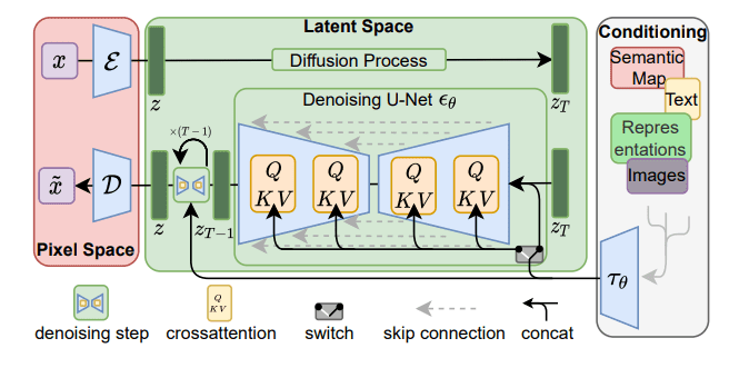
Figure 5:Latent diffusion model architecture.
Encoder: Transforms high-dimensional images into a compact latent representation.
Decoder: Reconstructs images from the latent representation.
The latent space in SDXL is a tensor with dimensions 4×64×64, capturing essential semantic features of the image[13][14].
Two-Stage Generation Process
The image generation process in SDXL follows a two-stage approach:
Compression: The VAE encodes the input image into the latent space.
Diffusion and Denoising: A U-Net-based diffusion model operates within the latent space, gradually transforming random noise into a coherent image representation guided by text prompts.
This method allows for efficient computation and detailed image generation[15].
Cross-Attention Conditioning
SDXL uses a cross-attention mechanism to integrate text prompts into the image generation process. The text prompts are encoded using a pre-trained CLIP model, and these embeddings guide the denoising steps in the diffusion process[16]. This enables precise control over the generated image’s content based on the provided text[15].
The cross-attention mechanism:
Aligns image features with text features
Weighs different parts of the image based on text relevance
Guides the denoising process to match the text description
The key points are:
Text embeddings guide both training and inference
Cross-attention connects text and image features
The process gradually refines random noise into matching images
The same architecture handles both processes, just in different directions
Latent Space Properties
The latent space in SDXL exhibits several notable properties:
Smoothness: Facilitates continuous transitions between different image concepts, allowing for gradual changes and interpolations[17].
Disentanglement: Enables the independent manipulation of specific image attributes, such as color or shape, without affecting other aspects[18].
Semantic Structure: Encodes high-level information, enabling the model to generate complex visual concepts from textual descriptions[19].
Recent Enhancements
Recent research focuses on improving the latent space’s properties and the generation process, including:
Smooth Diffusion: Creating smoother latent spaces to enhance performance in image synthesis tasks[20].
Textual Inversion and Concept Injection: Enhancing control over specific visual concepts by manipulating directions within the latent space[19].
These advancements contribute to more efficient and higher-quality image generation, providing users with greater control and flexibility.
Resources
Introduction to Diffusion Models for Machine Learning - Assembly AI - A beginner-friendly deeper dive into diffusion models for machine learning.
Understanding the Latent Space of Diffusion Models - NIPS papers Understanding the Latent Space of Diffusion Models - NIPS papers - A deeper dive on latent space for diffusion models.
Stable Diffusion GitHub Repo - Official repository for Stable Diffusion XL. You can find the latest code, models, and documentation here.
Diffusion Models for Image Generation - OpenAI - A comprehensive overview of diffusion models and their applications in image generation.
Step by Step Visual Introduction to Diffusion Models - A visual guide to understanding diffusion models, including the mathematical concepts involved.
References
Here are the references used in this guide: